Quantum computing basics part 1

Learning quantum computing (which I abbreviate as QC in this series’ titles) can be, and often is, challenging. One of the common problems is finding resources that help learning the basics with some practical examples (and not only mathematical equations). This inspired me to start a series of articles that cover exactly this — quantum computing basics — with focus on coding them with Qiskit. You can find all the articles under the #qcbasics hashtag.

In this post I write about Pauli operators — one of the most important single-qubit operators available for quantum programmers. They are used for the most common qubit operations, they form measurement bases, and they are absolutely crucial for quantum error correcting codes, among other things. They are also simple enough to be a great starting point.

Defining Pauli operators

There are four Pauli operators: identity, bit-flip, bit-and-phase-flip, and phase-flip. They are represented with the following symbols: ${"font":{"size":11,"family":"Arial","color":"#000000"},"aid":null,"backgroundColor":"#ffffff","id":"1","code":"$$\\mathbb{I}$$","type":"$$","backgroundColorModified":false,"ts":1772710460915,"cs":"PBtLbk5xx0EER9KhBoxrtg==","size":{"width":5,"height":10}}$ , X, Y, and Z. We will look at them in detail in a moment. But let me cover their common properties before.

They are all represented by 2 ⨉ 2 matrices. Such matrices are called square matrices. All Pauli operators are also unitary matrices.

Unitary matrices

A unitary matrix is a matrix that is invertible, which means that its inverse (U^-1) is equal to its conjugate transpose (U*). What does it mean? Let us take the X operator as an example.

On the left-hand side you can see X’s reverse, and on the right-hand side X’s conjugate transpose.

(If you do not know how to calculate those, you can use this calculator.)

Finally, a unitary matrix must satisfy the following condition as well — a product of the matrix itself and its conjugate transpose must be equal to the identity matrix.

Generally, all quantum operators must be unitary, since everything that happens in a quantum processor must be reversible.

Hermitian matrices

All Pauli operators are also Hermitian matrices. It means that they are equal to their own conjugate transpose. Following the previous example with the X operator, let us take a look at the following example.

This one was easier, was it not?

Anti-commuting

Each Pauli operator anti-commutes with each other (except for the identity operator). Fancy wording, but what does it mean? If a mathematical operations anti-commutes it means that swapping the position of two arguments of an this operation gives a result which is the inverse of the result with unswapped arguments. In case of the Pauli operators it looks like the following:

Multiplication

The Pauli operators multiply as any other square matrix, but I listed the multiplication rules here in case you would need them.

stands for an imaginary part of a complex number.

The identity operator

We covered all the properties of Pauli operators, but we have not taken a look at the operators themselves. Let us begin with the identity operator, the only operator that is actually trivial in this set as it does nothing to the state of a qubit. The matrix for this operator looks like the following.

I promised practical examples, and the time has come to code something. All the examples in this article follows the same template:

Define a |1⟩ qubit.
Define a quantum circuit with the demonstrated operator as a gate, and visualise it.
Define a quantum circuit with the demonstrated operator as an operator, and visualise it.

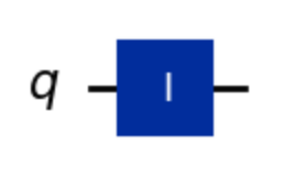
The most common way of using this operator is as a gate, like in the following example.

qc = QuantumCircuit(1)
qc.id(0)

Qiskit, however, allows for more complicated usage of Pauli operators using a dedicated class, and circuit appending instead.

qc = QuantumCircuit(1)
i_operator = Pauli('I')
qc.append(i_operator, [0])

In any case, the circuit looks like below and yields |1⟩ as the result.

The bit-flip operator

The identity operator is indeed trivial, so let us switch to something that actually does something — the bit-flip, or X operator. It does something relatively simple, namely reverses whatever the value of a qubit is. It is characterised by the following matrix.

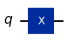
Here is how the operator looks like as a gate.

qc = QuantumCircuit(1)
qc.x(0)

And the corresponding operator part.

qc = QuantumCircuit(1)
x_operator = Pauli('X')
qc.append(x_operator, [0])

In both cases, the result of this operation is |0⟩, and the circuit looks like the following.

The phase-flip operator

The next operator — the bit-flip or Z operator — does the same thing to the phase as the X operator does to the bit value. It flips it. The trick is that it is not visible in the classical readout operation that one usually applies to see the results. The state is purely quantum, and cannot be directly translated. It is defined by the following matrix.

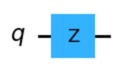
When coded as a gate, it looks like this.

qc = QuantumCircuit(1)
qc.z(0)

And here as an operator.

qc = QuantumCircuit(1)
z_operator = Pauli('Z')
qc.append(z_operator, [0])

In both cases again, the result is the same. It is |-⟩ (would be |+⟩ if the input was |0⟩). And in the diagram.

The bit-and-phase-flip operator

Last but not least, we have the bit-and-phase or Y Pauli operator. It is sort of a mixture of the X and Z operators, since it does both things. Remember, however, that only the bit-flip part can be measured classically, as the phase part is lost during a readout. Here is the matrix.

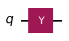
If we implement it as code, we do it in the following way.

qc = QuantumCircuit(1)
qc.y(0)

And similarly as an operator.

qc = QuantumCircuit(1)
y_operator = Pauli('Y')
qc.append(y_operator, [0])

The result we get is |-i⟩ (would be |i⟩ if the input was |0⟩). The diagram is as follows.

Operators in Qiskit

Gates in Qiskit are handy functions that allow one to create circuits quickly, but abstract away a lot of details and low-level functionality. Defining circuits with operators is much more verbose, but allows implementations which are more detailed and flexible. I will not dig into the details here, since it is a broad topic which deserves its own article (or a book, actually). However, below you can find a sample code snippet that will give you a glimpse of their capabilities.

# Multi-qubit Pauli (Z ⊗ X on two qubits): Z on qubit 0, X on qubit 1.
pauli_zx = Pauli('ZX')

# Convert to Operator for matrix math.
op_x = Operator(pauli_x)
print(op_x.data)

# Check commutation.
print(pauli_x.compose(pauli_z).commutes(pauli_z.compose(pauli_x)))

Summary

The Pauli operators are one of the most basic building blocks of quantum circuits, gadgets and algorithms. There are four of them: ${"font":{"size":11,"family":"Arial","color":"#000000"},"aid":null,"backgroundColor":"#ffffff","id":"1","code":"$$\\mathbb{I}$$","type":"$$","backgroundColorModified":false,"ts":1772710460915,"cs":"PBtLbk5xx0EER9KhBoxrtg==","size":{"width":5,"height":10}}$ , X, Y, and Z, also called the identity, bit-flip, bit-and-phase-flip, and phase-flip operators. Each of them is represented with a square matrix that is both unitary and Hermitian.

The operators can be used on a single qubit in Qiskit either as gates, or operators. The gate representation allows us for faster implementation, and cleaner code, but the operator representation gives us power over the low-level implementation details, and more flexibility.

Overall, the Pauli operators are something that any quantum developer must be familiar with, as they are virtually in any quantum circuit we will ever build. Even if we do not use them explicitly, they are the foundation of modern-day error-correction codes that allow us to use qubits reliably.