Visualisation of circuits

Quantum computing basics part 2

A picture is worth a thousand words. This old saying holds true in almost any subject one can think of. It is no different when it comes to implementation of quantum circuits. Visualisation of circuits can be crucial, especially when you build bigger, more complicated ones. It may be much easier to understand what they do, and why they yield these (and not other) results when looking at their diagrams instead of the code that brought them to life. In this post I will walk you through the most common use cases in circuit visualisation.

I use Qiskit as the quantum framework of choice, and the code you see here is written in Python.

A simple circuit

You cannot visualise something that does not exist, so let us start with a rather simple circuit that we are going to use through most of this article.

circuit = QuantumCircuit(3, 3)
circuit.h(range(3))
circuit.x(0)
circuit.cz(0, 1)
circuit.x(2)
circuit.measure(range(3), range(3))

Simple draw

So, what does this circuit do? Looking at the code, you can tell that it applies a Hadamard gate to all the qubits, then a NOT gate to the first qubit, a control-Z gate to the first and second qubits, and finally a NOT gate to the last qubit. Then a measurement is performed on all the qubits. But in order to tell it, you must remember how the range() function works, and how the qubits are ordered in Qiskit. It would be much easier to not have to rely on all this knowledge, would it not?

Qiskit has a lot of sophisticated functionality as far as drawing the circuits goes, but it is also vital to know the basics. After all, all that functionality relies on packages and software that may not be available to you all the time. The first and simplest way to get a circuit print is to pass it to the print() function.

print(circuit)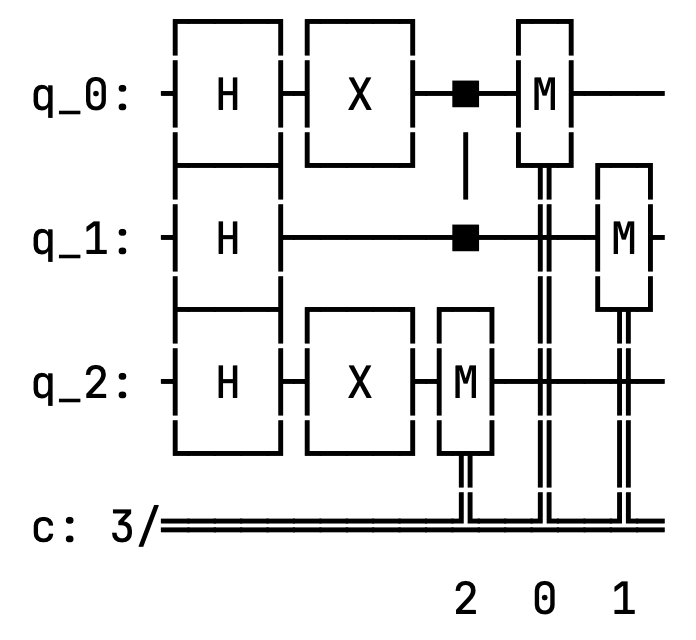

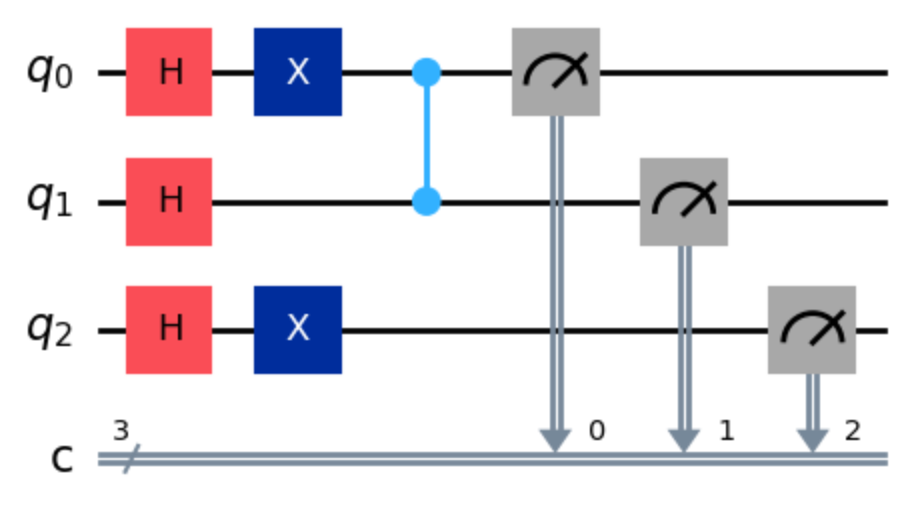
It is not pretty, but it works. A slightly better result can be achieved by calling the draw() function on the circuit object.

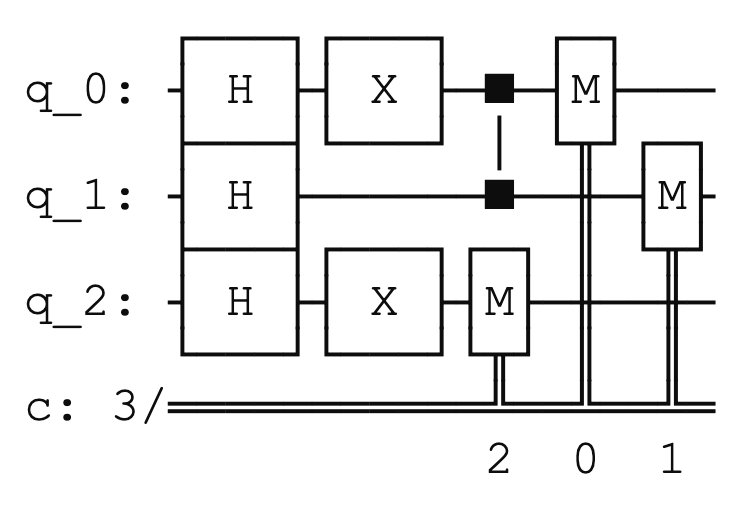
This one looks much better. But can we even get better than this?

Rendering engines

Qiskit supports external rendering engines. A rendering engine is a software component responsible for converting data (like vector graphics, text, or 3D models) into a visual output (e.g., images, animations, or interactive displays). It handles tasks like drawing shapes, applying colors, managing fonts, and rendering layouts. You can use those engines to get better circuit diagrams than the simple draw allows for.

The less popular, but more capable, engine is LaTeX. It is a separate software package that must be installed independently on the system. If you use a MacBook like me, you can get a copy here. Additionally, you must ensure that your project uses the qcircuit package. Then you can select the LaTeX backend as your rendering system this way:

circuit.draw(output="latex")

The most popular engine is Matplotlib. I guess it is because its capabilities are fairly decent, but it is much easier to install, and manage. You just have to install the pylatexenc and matplotlib packages in your virtual environment (or Jupyter server), and you are good to go. Then you can print the circuit using the following command.

circuit.draw(output="mpl")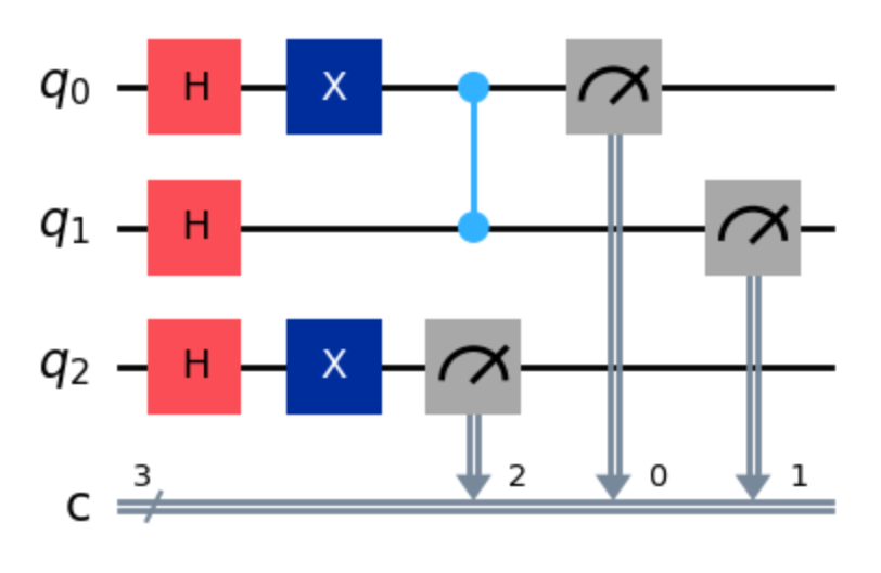

This one looks much better, does it not?

I will use Matplotlib in the rest of the examples in this article, but if you wish to use LaTeX instead, just change the value that you pass to the output parameter.

How does the  `draw` function work?

Normally, the  draw method returns the rendered image as an object and prints nothing.

Which class it returns depends on the output you specify: the default  ’text’  yields a  TextDrawer,  ’mpl’  yields a  matplotlib.Figure, and  ’latext’  yields a PIL.Image object. Jupyter notebooks recognise these return types and display them automatically, but outside of Jupyter the images will not appear on their own. So do not be surprised that nothing is drawn if you use a vanilla Python environment.

Saving the output

So far so good, but apart from visual inspection, the figures that we have plotted are not for much use. Sure, you can make print screens of them to include them in your documentation, or share around, but it will soon become cumbersome, or not really feasible (especially, if your circuits get bigger and bigger). Luckily, you can save the render to a separate file.

Sometimes our circuits can get quite big. Jupyter does its best to fit them in the available space, but it can be useful to save the diagram as an image file. The draw method has an optional argument filename that allows us to specify the name of the file where to save the diagram. The file format is inferred from the extension of the filename, and it can be any format supported by Matplotlib, such as PNG, PDF, SVG, etc. This way you can save the diagram in a high-quality format that can be easily included in reports, presentations, or publications, or just enlarge it to see the details more clearly.

circuit.draw(output="mpl", filename="circuit-mpl.png")

By default the file is saved to the current working directory, but you can provide a relative or an absolute path if you wish to override this behaviour.

circuit.draw(output="mpl", filename="./img/circuit-mpl.png")

Additional controls

Interactivity

Interactivity is actually a big word for what is available in circuit plotting. When you call the  draw function using either Matplotlib or LaTeX as the render engines, you can pass the interactivity=True argument in the  kwarg parameter. It will cause the drawing to be opened in a new window. It has one downside though. It does not work in Jupyter notebooks so well.

Barriers

Barriers are a very useful tool in bigger circuits, but they can be effectively demonstrated in our small circuit too. Let us rewrite it adding two barriers to it.

circuit = QuantumCircuit(3, 3)
circuit.h(range(3))
circuit.barrier()
circuit.x(0)
circuit.cz(0, 1)
circuit.x(2)
circuit.barrier()
circuit.measure(range(3), range(3))

Calling the circuit.draw(output="mpl") function will give us the following result.

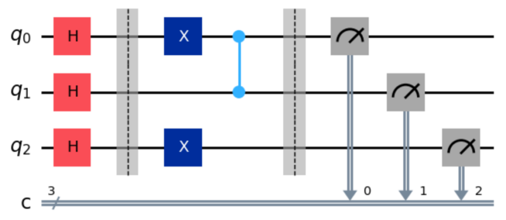
The barriers are those two vertical, grey bars. They do not have any logical effect on the circle, but allow us to visually group distinct parts of it.

Some circuits come in with built-in barriers. This can be the case when you use a quantum primitive, or you append sub-circuits to a bigger one. They are there to distinguish distinct parts of the super-circuit. But sometimes they may be in the way of what you are trying to achieve. You can disable them with the following line of code.

circuit.draw(output="mpl", plot_barriers=False)

In the case of our modified circuit we will get the following result.

Sure, in the case of our circuit it does not really make sense to disable the barriers that we put there ourselves, but, as I wrote, sometimes you do not control the code of the circuit, but would still like to get rid of the additional separators.

Reversing the qubits

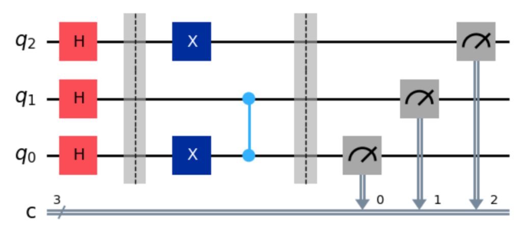
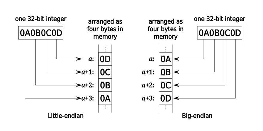
Qiskit uses little endian by default. If you do not know what I am writing about right now, please check a dedicated post on it that I published a while ago. This, however, may be in the way of how you want to visualise the data. You can easily reverse the order of the qubits in the render with this line.

circuit.draw(output="mpl", reverse_bits=True)

As you can see, the qubits are listed now from the last (and not first) index at the top.

Styling

Surprisingly enough, Matplotlib supports providing custom styles to the rendering engine. You can create a style object (using a syntax known from CSS), and then pass it to your drawing function like in the following example.

background = {"backgroundcolor": "lightblue"}
circuit.draw(output="mpl", style=background)

It will obviously change the background colour to light blue.

You can also steer the scale of the image by setting the scale parameter of the draw function, like in the following example:

circuit.draw(output="mpl", scale=0.3)

This may help visualising bigger circuits in Jupyter notebooks by shrinking them.

Folding

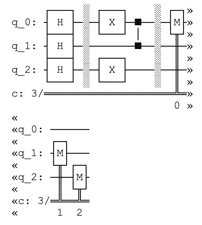
Folding was a very popular technique of managing the output of programs back in the days where command line interfaces were prevalent. You can still see it in action today if you use tools like AWS CLI. It serves the same purpose in Qiskit. If you use the text rendering engine, and you have strict display size limitations, you can fold the output to the next line like this:

circuit.draw(output="text", fold=30)

The result looks somewhat funny, with the double arrows indicating the folding line. I do not recall using it before doing the research for this blog post, but I hope this trick may save you one day.

Standalone function

Last but not least, Qiskit allows printing circuits without invoking functions on them. There is a standalone function circuit_drawer that effectively does the same as the draw function from the QuantumCircuit class. You have to import a separate package — qiskit.visualization — in order to benefit from it, but otherwise the usage is quite straightforward.

from qiskit.visualization import circuit_drawer
circuit_drawer(circuit, output="mpl")

The function supports all of the parameters and print options that I discussed in this article, and I encourage you to experiment a bit with it.

Conclusion

Visualisation is not a luxury, it is a necessity when you start to juggle more than a handful of qubits or when you need to communicate your ideas to others. In Qiskit the draw method is the gateway to a rich set of tools that let you switch between a quick text preview, a tidy Matplotlib image, or a high‑resolution LaTeX output with a single line of code. You can even open the figure in a separate window, drop in barriers to group logical blocks, reverse the qubit order to match your intuition, and customize colours, scale or background with a few dictionary entries. If you prefer a more imperative style, the circuit_drawer helper gives you the same flexibility without having to touch the circuit object itself.

Beyond the aesthetics, these visual aids help you spot mistakes, understand interference patterns, and explain the behaviour of your circuit in papers, slides or notebooks. The ability to fold long text outputs, to save diagrams in vector formats, and to toggle optional features like barriers means you can adapt the same code to a wide range of audiences and display constraints.

Circuit visualisation is just a beginning, a step that you should remember before submitting your circuit to run on a simulator or real hardware. But the journey does not end here. In the next part of this series we will take a look at visualising computation results.

Pauli operators

Quantum computing basics part 1

Learning quantum computing (which I abbreviate as QC in this series’ titles) can be, and often is, challenging. One of the common problems is finding resources that help learning the basics with some practical examples (and not only mathematical equations). This inspired me to start a series of articles that cover exactly this — quantum computing basics — with focus on coding them with Qiskit. You can find all the articles under the #qcbasics hashtag.

In this post I write about Pauli operators — one of the most important single-qubit operators available for quantum programmers. They are used for the most common qubit operations, they form measurement bases, and they are absolutely crucial for quantum error correcting codes, among other things. They are also simple enough to be a great starting point.

Defining Pauli operators

There are four Pauli operators: identity, bit-flip, bit-and-phase-flip, and phase-flip. They are represented with the following symbols: ${"font":{"size":11,"family":"Arial","color":"#000000"},"aid":null,"backgroundColor":"#ffffff","id":"1","code":"$$\\mathbb{I}$$","type":"$$","backgroundColorModified":false,"ts":1772710460915,"cs":"PBtLbk5xx0EER9KhBoxrtg==","size":{"width":5,"height":10}}$ , X, Y, and Z. We will look at them in detail in a moment. But let me cover their common properties before.

They are all represented by 2 ⨉ 2 matrices. Such matrices are called square matrices. All Pauli operators are also unitary matrices.

Unitary matrices

A unitary matrix is a matrix that is invertible, which means that its inverse (U^-1) is equal to its conjugate transpose (U*). What does it mean? Let us take the X operator as an example.

On the left-hand side you can see X’s reverse, and on the right-hand side X’s conjugate transpose.

(If you do not know how to calculate those, you can use this calculator.)

Finally, a unitary matrix must satisfy the following condition as well — a product of the matrix itself and its conjugate transpose must be equal to the identity matrix.

Generally, all quantum operators must be unitary, since everything that happens in a quantum processor must be reversible.

Hermitian matrices

All Pauli operators are also Hermitian matrices. It means that they are equal to their own conjugate transpose. Following the previous example with the X operator, let us take a look at the following example.

This one was easier, was it not?

Anti-commuting

Each Pauli operator anti-commutes with each other (except for the identity operator). Fancy wording, but what does it mean? If a mathematical operations anti-commutes it means that swapping the position of two arguments of an this operation gives a result which is the inverse of the result with unswapped arguments. In case of the Pauli operators it looks like the following:

Multiplication

The Pauli operators multiply as any other square matrix, but I listed the multiplication rules here in case you would need them.

stands for an imaginary part of a complex number.

The identity operator

We covered all the properties of Pauli operators, but we have not taken a look at the operators themselves. Let us begin with the identity operator, the only operator that is actually trivial in this set as it does nothing to the state of a qubit. The matrix for this operator looks like the following.

I promised practical examples, and the time has come to code something. All the examples in this article follows the same template:

Define a |1⟩ qubit.
Define a quantum circuit with the demonstrated operator as a gate, and visualise it.
Define a quantum circuit with the demonstrated operator as an operator, and visualise it.

The most common way of using this operator is as a gate, like in the following example.

qc = QuantumCircuit(1)
qc.id(0)

Qiskit, however, allows for more complicated usage of Pauli operators using a dedicated class, and circuit appending instead.

qc = QuantumCircuit(1)
i_operator = Pauli('I')
qc.append(i_operator, [0])

In any case, the circuit looks like below and yields |1⟩ as the result.

The bit-flip operator

The identity operator is indeed trivial, so let us switch to something that actually does something — the bit-flip, or X operator. It does something relatively simple, namely reverses whatever the value of a qubit is. It is characterised by the following matrix.

Here is how the operator looks like as a gate.

qc = QuantumCircuit(1)
qc.x(0)

And the corresponding operator part.

qc = QuantumCircuit(1)
x_operator = Pauli('X')
qc.append(x_operator, [0])

In both cases, the result of this operation is |0⟩, and the circuit looks like the following.

The phase-flip operator

The next operator — the bit-flip or Z operator — does the same thing to the phase as the X operator does to the bit value. It flips it. The trick is that it is not visible in the classical readout operation that one usually applies to see the results. The state is purely quantum, and cannot be directly translated. It is defined by the following matrix.

When coded as a gate, it looks like this.

qc = QuantumCircuit(1)
qc.z(0)

And here as an operator.

qc = QuantumCircuit(1)
z_operator = Pauli('Z')
qc.append(z_operator, [0])

In both cases again, the result is the same. It is |-⟩ (would be |+⟩ if the input was |0⟩). And in the diagram.

The bit-and-phase-flip operator

Last but not least, we have the bit-and-phase or Y Pauli operator. It is sort of a mixture of the X and Z operators, since it does both things. Remember, however, that only the bit-flip part can be measured classically, as the phase part is lost during a readout. Here is the matrix.

If we implement it as code, we do it in the following way.

qc = QuantumCircuit(1)
qc.y(0)

And similarly as an operator.

qc = QuantumCircuit(1)
y_operator = Pauli('Y')
qc.append(y_operator, [0])

The result we get is |-i⟩ (would be |i⟩ if the input was |0⟩). The diagram is as follows.

Operators in Qiskit

Gates in Qiskit are handy functions that allow one to create circuits quickly, but abstract away a lot of details and low-level functionality. Defining circuits with operators is much more verbose, but allows implementations which are more detailed and flexible. I will not dig into the details here, since it is a broad topic which deserves its own article (or a book, actually). However, below you can find a sample code snippet that will give you a glimpse of their capabilities.

# Multi-qubit Pauli (Z ⊗ X on two qubits): Z on qubit 0, X on qubit 1.
pauli_zx = Pauli('ZX')

# Convert to Operator for matrix math.
op_x = Operator(pauli_x)
print(op_x.data)

# Check commutation.
print(pauli_x.compose(pauli_z).commutes(pauli_z.compose(pauli_x)))

Summary

The Pauli operators are one of the most basic building blocks of quantum circuits, gadgets and algorithms. There are four of them: ${"font":{"size":11,"family":"Arial","color":"#000000"},"aid":null,"backgroundColor":"#ffffff","id":"1","code":"$$\\mathbb{I}$$","type":"$$","backgroundColorModified":false,"ts":1772710460915,"cs":"PBtLbk5xx0EER9KhBoxrtg==","size":{"width":5,"height":10}}$ , X, Y, and Z, also called the identity, bit-flip, bit-and-phase-flip, and phase-flip operators. Each of them is represented with a square matrix that is both unitary and Hermitian.

The operators can be used on a single qubit in Qiskit either as gates, or operators. The gate representation allows us for faster implementation, and cleaner code, but the operator representation gives us power over the low-level implementation details, and more flexibility.

Overall, the Pauli operators are something that any quantum developer must be familiar with, as they are virtually in any quantum circuit we will ever build. Even if we do not use them explicitly, they are the foundation of modern-day error-correction codes that allow us to use qubits reliably.

JavaZone 2025: A Speaker’s Perspective

I usually write about quantum computing, sometimes about Java and related things. However, fresh from my recent experience as a speaker on one of the largest European conferences (and one that’s marked as one of the best), I thought that you, dear Readers, may be interested in a slightly different article. This time I write about how it was to be one of the one hundred speakers on JavaZone 2025. I thought you may find it interesting to learn how to secure a spot at such a big event, prepare, and give it a go.

Let’s begin with some key facts. JavaZone 2025 took place 2^nd－4^th September 2025 in Lillestrøm, Norway. According to this database, it hosted 90 speakers, 150 exhibitors, and 2500 thousand attendees. It definitely felt crowded there, especially in the partners’ area. The first day actually took place in Oslo, and hosted exclusively workshops. The main two conference days, with presentations and lightning talks, were 3^rd－4^th September. There was one special event the day before: a dinner for the speakers. I couldn’t attend it due to personal reasons, but I quite regret it. It’d be a great opportunity to hang out with the others, since I didn’t actually have a chance during the conference days.

I gave a lightning talk titled “Quantum Leap with Java: An Unrealistic Dream?” You can find it recorded here. Be sure to watch at least a minute or two of it, since there’s one important thing I write about later. I think it was well received, though I didn’t get that much feedback, to be honest. Anyway, I’m quite happy with how I performed. And speaking of which, how did it actually go?

Getting a Spot

Nothing of this would’ve happened of course if I didn’t get a spot in the first place. It all started on 18^th February, when I got an email that a call for proposals was opened. This email isn’t sent to everyone, but if you’ve ever submitted, then you’ll get it unless you’ve unsubscribed yourself. This time it was actually my second time trying to get my talk accepted. Two years ago, in 2023 I submitted a longer form, a 45-minutes presentation about the modulith architecture and different libraries supporting it. It was rejected, but gave me quite a precious lesson on how to make a second attempt. For various reasons I couldn’t try last year, so I waited until 2025. The call for proposals ended 28^th April, and on 25^th June I knew mine was accepted. How did I secure it this time?

First of all, I realised that the modulith pattern might have been too weird to be accepted. After all, there’re many Java developers that have very bad memories when the word monolith is spoken aloud (me included). And though I believe that the modulith architecture is one of the best ever proposed (and quite different from the real monolith), it hasn’t actually gained any momentum until this year. Instead, I opted for something “sexier”. Quantum computing is definitely quite famous despite still being a niche thing. I started to learn it a year before submitting, so I was already well prepared to talk about it. Moreover, I’ve always been deeply concerned that Java developers are missing yet another opportunity to develop one of the great technologies of this decade (the second one being AI), so I thought it’s a great opportunity to hit two birds with one stone.

Second of all, a shorter form is easier to “squeeze in” in case your topic isn’t among the top contenders, but is still solid. Therefore I opted for a lightning talk instead of a presentation. Moreover, it suited my purpose better. Java libraries for quantum development are somewhat disappointing, and I didn’t see a big point in presenting what other languages are capable of at a conference having the word “Java” in its name. However, one of the purposes of lightning talks is to spread ideas, and in my case – alert our Java community. It’s beyond my competence to decide what we should do with the fact that Java is heavily lagging behind in the quantum race, but I felt obligated to shout it out anyway. Hence the choice of the form of lightning talk, which I believe worked quite well.

Once I’d made up my mind, it was time to apply. You have to fill a pretty long form in order to submit your talk. There you must provide a title for your speech and a publicly visible, short description. This is the abstract that ends up in the program eventually. There’s also a separate, longer program-committee-visible description. It’s to help its members evaluate your proposal. There you must provide a more detailed layout. I did it in the form of a list of bullet points, but there’s no style enforced whatsoever. You also have to specify the form of the “thing” (a presentation, a lightning talk or a workshop), duration, and language. I opted for English for two reasons. I speak it way better than Norwegian, and it made more sense given it’s an international conference. Finally, you must provide information about yourself, including a short bio, links to your online presence, and conference availability. For example, if you aren’t fully flexible, you can state it there.

There’s one caveat filling the form though. Sometimes it doesn’t get saved. So it’s safer to write the stuff down in some notepad, and then just paste and send, which is what I did.

Preparing the Talk

Regardless of what subject you have chosen, there’s one thing you must remember about above anything else: time. Every form of presentation is timeboxed, and the technical crew is pretty strict about staying within this limit. It means that you have to take extra care about the amount of material you want to show.

My rule of thumb is to prepare the stuff for only 75% of the available time. This gives me some safety margin in case I talk a bit too long about something or improvise an anecdote or two. I guess it happens to all speakers, especially when nerves and adrenaline kick in. Having those extra minutes can be a lifesaver. In the case of my talk, I planned to prepare the material for 15 minutes, and have 5 minutes just in case. The actual talk took me slightly longer than 18 minutes, so it worked pretty well.

The starting point for my preparation was the layout of the talk that I submitted a couple of months before. Don’t worry, it isn’t carved in stone. Speakers are allowed to modify their submissions, to some degree of freedom obviously. I’ve never done this, so I don’t have first-hand experience on how it goes.

Regardless of whether I prepare public talks, or courses, I always write down what I want to say. Exactly the way I’ll be saying it. This way is much easier for me to prepare for the actual event. It reduces the variability when repeating the talk during preparation, and helps me memorise the key points. When this is done, I do the slides too (or any other form of presentation, ex. code). With the whole “presentation pack” in place, I read it out loud trying to simulate actually giving it as much as possible with a stopwatch. The goal is to make it within the 75% of maximum time available. If I can’t make it most of the time, it means I’ve prepared too much material and have to edit it.

If I’m happy however with the way this part goes, then I use a highlighter to mark all the important keywords and parts of the talk. It’ll be crucial during the repetition phase, which is next. During it I read the talk aloud. I haven’t counted how many times I did it, but the point wasn’t to learn it by heart. It was on the other hand to memorise it enough to be able to give it smoothly even when I’m stressed or something unplanned happens.

Once I’m happy with it, I practise giving it the way I actually want to give the talk. With slides, code, and everything else. This helps me automate moments of switching the slides or live coding. Again, it’s to mitigate the stress ruining your talk. Why is it so important? I’m a pretty cool person, but still I always get a bit nervous when I talk during such events. I’m fairly certain that most of you have that too. Even if it isn’t a full blown stage fright, it may still ruin your talk. So I prefer not to take chances and just prepare well enough.

Finally, I “give” the speech with the stopwatch again. It’s just to double-check if I still make it in time after all this practice. If so, I take a couple of days just before the conference free from the talk, to let it sink in my head, and rest a bit. And last but not least, taking a good night’s sleep the night before the talk is crucial.

The Conference Day

The conference day is no less important than all the preparation before. I always make sure that the means of transport I take can take me well before the time of my talk. I wasn’t at the opening session on JavaZone, but still made it therebefore 10 o’clock. It was much earlier than my talk, that was a bit after 4 o’clock, but I wanted to attend some presentations, and hang out with friends. These are actually two traps that one can easily fall into.

Attending the presentations can be quite mentally exhausting. I always try to avoid participating in too many if I’m the speaker, so this time I also chose three I was the most interested in, and skipped the rest. You may be thinking that I was too harsh on myself, and could’ve attended more. However, it’s important to remember that the attendees are at the conference to take the most of the talks that’s possible. It’s a matter of professional ethic to be able to be at your tops when you’re giving a talk. That’s why I do my best to avoid cognitive overload, and that’s why I went to only the talks that I really wanted to attend.

One of the talks that I attended was in the room that mine was scheduled for later that day. JavaZone actually hosts a special walk around the day before the first day of the conference. It’s meant for the speakers to get familiar with the rooms and facilities. Unfortunately, I couldn’t attend it, so I had to rely on that little trick to know what the room looks like. I didn’t want to discover something surprising just before my talk.

The second trap is networking or hanging out with friends. Not because it can be tiresome. Usually it isn’t. However, talking for a couple of hours puts a huge strain on your throat. So while I really enjoyed time with them, I made sure that I have at least one hour of keeping my mouth shut, so the throat can rest.

What Went Well and What Went Wrong

Well, I got the spot. But more seriously, I believe that the choice of the form (lightning talk), and a “sexy” topic (at least I believe quantum computing can be considered one) contributed to getting my proposal accepted. I’ve learned that there were around 800 submissions, so only approximately one in eight got accepted. I’m not sure I wouldn’t fail to get a place again if I didn’t do it this time with a better strategy.

I’m also quite happy with the amount of preparation I put into the talk. It went pretty well despite I caught some nerves in the middle of talking (of course!). I’m fairly certain that if I hadn’t memorised it so well, I could’ve panicked or at least not given it so smoothly.

According to my estimation (which can be wildly wrong since I did it just on the stage, two minutes before the talk), there were about 20-30 people in the audience. Given the relatively late time, I think the talk was still fairly popular. I may as well be deluding myself, but I’m anyway satisfied with this.

And last but not least, I actually got some feedback and follow-up questions. The feedback was generally positive, though I also got some remarks about stuff I should work on if I’m to give yet another talk. It’s actually quite valuable, I like to take every chance to improve my skills. Plus, it showed me that there were at least a couple of people that were genuinely interested in the talk.

That would be it when it comes to the positive things. And now to the downsides. First of all, despite being wary of not showing too early, and conserving my energy, I failed to do this. I really wanted to hang out with friends, and attend some talks, but in turn it made me more tired than I wished. It wasn’t good from the talk’s perspective, so I definitely should’ve worked a bit on balancing this one out. But on the other hand, it’s hard to just turn your folk down, so I may as well repeat the same thing again.

That would be more on perfecting my performance. But there was something that I really screwed up, and didn’t realise until it was way too late. I have eye comfort settings turned on on my devices almost all the time. The lights in the rooms at Nova in Lillestrøm were quite warm, so I haven’t turned it off. After connecting I check if the presenters screen is in neutral color, which was. This was to ensure that the presentation will also be displayed without any filter on. But I didn’t think that the software they used for recording my presentation would also pick up the warm colour that the eye comfort shield bathed my display with. When you look at the slides in the Vimeo recording, you’ll see that they have an unnaturally warm tone. I haven’t confirmed it with JavaZone organisers, but I’m fairly certain that it’s because of my settings. Next time I do have to remember to turn this off no matter what to avoid peach vibes emanating from the slides.

Conclusion

It was really a great experience to give a lightning talk at this year’s JavaZone. I really enjoyed it, and I hope my audience did too. I wouldn’t be there, if not for the carefully prepared strategy for picking up the topic and the form of presentation. I also spend a lot of time preparing for it, so I can give it as professionally as possible regardless of conditions or my psychological state. The most important thing was to be mindful of the time limit at every stage of preparations, but proper repetition did its job too.

The talk went quite well, and I’ve got enough positive feedback to call it a success. Despite overestimating my stamina, I avoided most of the pitfalls of all the things that surrendered my talk. However, one can never be overprepared. My eye comfort settings badly affected the way the slides were recorded, effectively downgrading the experience of anyone watching my talk on Vimeo. This is something to work on in the future.

Finally, this isn’t meant to be a guide on how to be a speaker at JavaZone (or any bigger conference as a matter of fact). However, if you find this article useful in your preparations, I couldn’t be happier.

Quantum Computing in Java

If you are new to quantum computing, then the title of this post will not sound suspicious or provocative to you. However, if you are a seasoned quantum user then you will know that something must be off here. After all, your language of choice is most likely Python, or maybe C if you are working on high-performing solutions.

The majority of frameworks and libraries in the field of quantum computing are written in Python, and made for this language. I am thinking of Qiskit, Ocean, and cirq, among others. There is a big ongoing effort by IBM to develop a parallel Qiskit framework for the C language, and one can even try Q# from Microsoft. What they have in common is comprehensive functionality, big company backing, and integration with real quantum hardware (to different extents, though).

But what about Java? Is it even possible to do any useful quantum development in this language? For a big part of my career I have been a Java/Kotlin developer, so this question is somewhat personal to me. And the answer is… it is complicated. There are two libraries that I have managed to find, and two JEPs that are focused on quantum computing. How useful are they? Let us find out.

JQuantum

The first library we are going to take a look at is called JQuantum. If you click on the link the first thing you will notice is that it has not been updated since 30^th July 2018. Being so outdated does not make it a candidate for any production project. Can it be of any use anyway?

JQuantum contains implementation of basic quantum computing concepts. You can find there classes for qubits, gates, circuits, and even the most famous algorithms like Grover’s algorithm or Shor’s algorithm.

Sadly, the library does not have any form of a simulator, not to mention the possibility to run the code against a real QPU. You can run your programs and output their results, but what JQuantum does behind the scenes is just linear algebra on vectors and matrices. Since the amount of memory necessary to contain multidimensional matrices scales exponentially, the amount of qubits you can use in JQuantum is severely limited. After all, even the simplest gates are two-dimensional matrices, and adding each qubit effectively doubles the number of dimensions in the matrix that represents such a system.

Okay, so the library is outdated, and its functionality is quite limited. Can we put it to any use then? In fact, we can. Let us take a look at a sample code.

class JQuantumExample implements Example {
    @Override
    public void show() {
        var qubitValue = 0;
        var quantumRegister = new QubitRegister(1, qubitValue);
       
        var notGate = QuantumGate.X;
        notGate.accept(quantumRegister);
        var measurement = quantumRegister.measure();
       
        System.out.println("JQuantum Example");
        System.out.println("----------------");
        System.out.println("Applied X gate to |" + qubitValue + "⟩; result is |" + measurement +"⟩.");
        System.out.println();
    }
}

In the code snippet above, we first create a qubit in the |0⟩ (read 0-ket) state. If you do not know what kets are, please read my post about them. Then, we create a quantum register (processor’s memory) with one qubit. We instantiate a NOT gate, often called an X gate. Then, we apply the X gate to the register, effectively flipping the value of the qubit from |0⟩ to |1⟩. Finally, we measure.

The measurement in quantum computing is an act of “translating” the result of the computation from quantum encoding to classical (i.e. binary) encoding. Thus, whatever is yielded by the program, ends up as either |0⟩ or |1⟩. Any other quantum state (and there is an infinite number of them) cannot be processed then by classical computers.

This code may not earn you any money, but it can still demonstrate basic principles of quantum programs. And this is what the JQuantum library is great for: education. If you have never written a line of code in any language other than Java, you can still learn a solid piece of quantum computing with this library.

If you would like to run this program you must add the Quantum.jar file to your classpath. You can find it in the root tree in the JQuantum’s repository.

Strange

If you are a Marvel fan, then you may be disappointed that I will not be writing about your favourite doctor here. Instead, Strange is the name of a quantum library written for the book Quantum Computing in Action by Johan Vos.

Strange is an open-source learning resource that can be used alongside the aforementioned book, or by itself. It is available via Maven Central, so no manual installation is needed like it was the case with JQuantum.

It has somewhat similar functionality to that library. You will find abstractions for qubits, gates, circuits (under the name of programs), and quantum algorithms. The collection is a bit smaller than in JQuantum, though.

On the upside, Strange does contain a quantum simulator. It is a simple one, without any sophisticated features of modern-day simulators (like noise or hardware-specific characteristics), but it can still be pretty useful. There are traces in the code that cloud integration was in progress, but it has never been finished. Thus, you cannot run code written with Strange on any actual quantum hardware.

Let us take a look at a code example.

public class StrangeExample implements Example {
   @Override
   public void show() {
       var qubitValue = 0;
       var program = new Program(1);
       var x = new X(qubitValue);

       var negationStep = new Step();
       negationStep.addGate(x);
       program.addStep(negationStep);

       var executionEnvironment = new SimpleQuantumExecutionEnvironment();
       var result = executionEnvironment.runProgram(program);
       var measurement = result.getQubits()[0].measure();
       
       System.out.println("Strange Example");
       System.out.println("---------------");
       System.out.println("Applied X gate to |" + qubitValue + "⟩; result is |" + measurement +"⟩.");
       System.out.println();
   }
}

This program does exactly the same thing as the previous one, and the first three steps are almost identical. The difference starts from the definition of a step. Steps are phases of a circuit, which is called a program in Strange. So in order to code the negation, we must first define a step for it (negationStep) and then add it to the program with the addStep method. Next, we have to instantiate the simulator in the form of executionEnvironment. Finally, we can run it, and obtain a measurement from the result.

Though JQuantum and Strange are very alike, the functionality of Strange is somewhat more robust. Both, however, are great learning resources for quantum computing newbies. Unfortunately, doing any real-life project with Strange is as unfeasible, as with JQuantum.

Post-quantum Cryptography

Believe it or not, but quantum computers are going to break all the cryptography that we use on an everyday basis. SHA, RSA, Diffie-Helman, and related protocols are useless against the codebreaking capabilities of future quantum computers. Luckily, they are not here yet. Even more luckily, I will spare you all the difficult math related to this issue.

Although quantum computers with enough qubits to run Shor’s algorithm for the inputs of size of nowadays use cryptographic keys are still at least a couple of years away, cryptographers have already started working on cryptographic protocols that are quantum-safe. By this they mean that they cannot be cracked by any kind of quantum computer or algorithm (at least for now). Why do they do this? There is an old attack pattern that relies on evasedropping the data now for later decryption. If an attacker follows it it can for example steal the packets in which you authenticate with your bank in hope of decrypting them whenever possible and obtaining your credentials. It may seem futile at first, but if a feasible quantum computer arrives in two years, then a lot of this data may still be valid. After all, how often do you rotate your bank password?

I mentioned that the cryptographers have already begun working on a solution. It arrived in the form of NIST standards in August 2024. Shortly after that, two JEPs were published: 496 and 497. The first one provides implementation for cryptographical keys creation and encapsulation. The second one is very similar, but can be used for signing, not encrypting keys. They can be used in the following way.

class PostQuantumCryptographyExample implements Example {
   @Override
   public void show() {
       try {
           var mlKem = "ML-KEM";
           var encryptionKeyGenerator = KeyPairGenerator.getInstance(mlKem);
           encryptionKeyGenerator.initialize(NamedParameterSpec.ML_KEM_512);
           var encryptionKeys = encryptionKeyGenerator.generateKeyPair();

           System.out.println("Post-Quantum Cryptography Example");
           System.out.println("---------------------------------");

           var publicEncryptionKey = encryptionKeys.getPublic().getEncoded();
           String publicKeyBase64 = Base64.getEncoder().encodeToString(publicEncryptionKey);
           System.out.println("Public key generated with " + mlKem + ": " + publicKeyBase64);

           var mlDsa = "ML-DSA";
           var signingKeyGenerator = KeyPairGenerator.getInstance(mlDsa);
           var signingKeys = signingKeyGenerator.generateKeyPair();
           var privateSigningKey = signingKeys.getPrivate();

           var helloWorld = "Hello World";
           byte[] message = helloWorld.getBytes();
           Signature signature = Signature.getInstance(mlDsa);
           signature.initSign(privateSigningKey);
           signature.update(message);
           byte[] signedMessage = signature.sign();

           System.out.println("Message \"" + helloWorld + "\" signed with " + mlDsa + ": " + Base64.getEncoder().encodeToString(signedMessage));
       } catch (NoSuchAlgorithmException | InvalidAlgorithmParameterException | InvalidKeyException |
                SignatureException e) {
           throw new RuntimeException(e);
       }
   }
}

If you have ever used other cryptographic keys in Java, then I am quite sure this code feels familiar to you. I will not describe it in detail here, since there is nothing related to quantum computing in it. We cannot use these implementations for working with qubits, gates or circuits. In fact, they do not even require a quantum computer to run. Instead, they rely on lattice structures that are immune to Shor’s algorithm since they do not use big primes multiplication.

Conclusion

While Java may not be the first choice for quantum computing due to the lack of robust, up-to-date libraries and frameworks, there are still learning resources available for those interested. The JQuantum and Strange libraries, although outdated or limited in functionality, can serve as valuable educational tools for beginners.

Moreover, with the impending threat of post-quantum cryptography being broken by future quantum computers, Java has already started addressing this challenge through JEPs 496 and 497. These provide implementations for creating and encapsulating cryptographic keys, ensuring our data remains secure even in a post-quantum world. Although they cannot be used for general quantum computing, they should at least provide a cornerstone for reliability of Java application in the quantum era.

While Java may not be the language of choice for quantum computing today, it is still possible to learn basic principles and prepare for a future where quantum-safe cryptography becomes the norm.

You can find all the code examples on my GitHub.

Post Scriptum

If you are interested in the prospects of quantum computing in Java and its future, I warmly invite you to join me on JavaZone2025 in Lillestrøm, Norway where I’ll give a lightning talk titled Quantum Leap with Java: An Unrealistic Dream? You can keep an eye on the program here. I am hoping to see you there!

Quantum Teleportation: A Step-by-Step Guide

Designing quantum circuits may seem a challenging task, but the longer one does it, the easier it gets with another approach. However, there is one thing that remains a problem regardless of how experienced you are with quantum computing – moving a state from one qubit to another.

In classical computing, you can simply read the result of your computations mid-air, copy it to another set of bits, and carry on like nothing happened. It is, physically, impossible to do in quantum computing, though. A theorem, known as the No-Cloning Theorem, explains why.

The No-Cloning Theorem is a fundamental principle in quantum mechanics, which states that it is impossible to create an identical copy of an arbitrary unknown quantum state. In simpler terms, you cannot duplicate an unmeasured qubit like you would with classical bits. I will save you the precise math that underpins it. What is important to remember, though, is that it is related to the destructive nature of the READ operation in QPUs. One cannot copy without reading what is to be copied in the first place. And reading a QPU result inevitably destroys any quantum state that was there, leaving only the classical result in the process.

Fortunately, a protocol exists that allows us to “move” an arbitrary quantum state from one qubit to another without destroying it. It is called quantum teleportation.

What the Teleportation Actually Means

No, unfortunately we will not feel like Spock from Star Trek. Nor will our qubits. Quantum teleportation is actually quite a misleading term. It does not instantly move matter from one place to another. It does not even do it with any information we may wish to transfer. It is much more grounded.

Quantum teleportation is a protocol that allows a sender (let her be Alice) to transmit a qubit to a receiver (let him be Bob) using a shared entangled quantum state and two bits of classical communication.

The protocol assumes Alice and Bob share an e-bit in the state |𝜙+⟩. The e-bit (entangled bit) in quantum computing refers to a quantum state that is shared between two parties and exhibits correlations that cannot be explained by classical physics. The state of an e-bit is represented in one of the Bell states. This shared state is essential for various quantum information processing tasks, including, unsurprisingly, quantum teleportation.

The e-bit could have been prepared in the past or through a third party or complex distributed process. Either way, how they both obtain the Bell state is of no concern to the protocol.

In addition to her part of the e-bit, Alice possesses a qubit Q that she wishes to transmit to Bob. Its state is unknown to both parties, and it may be entangled with other systems they cannot access. It is also important that the quantum teleportation protocol is only worth considering if physically sending the qubit Q to Bob is considered infeasible, for example because the quantum system would decohere before it reaches its destination. Alice can send classical information to Bob, though.

Remember that it is not possible to transmit quantum information using classical communication alone due to the no-cloning theorem. However, with the shared e-bit in place, Alice and Bob can accomplish their task through the quantum teleportation protocol.

As you can see, quantum teleportation, despite a fancy name, is just a protocol allowing for sending quantum information using entanglement and classical communication over arbitrary distances. Let us take a look at it.

The Protocol

The protocol involves a couple of steps which I will walk you through in order to get a good grasp of the topic. And nothing helps learning like a good visualisation of the subject.

The protocol consists of the following steps.

Alice performs a controlled-NOT operation on the pair (A, Q), with Q being the control and A being the target, and then performs a Hadamard operation on Q.
Alice then measures both A and Q, with respect to a standard basis measurement in both cases, and transmits the classical outcomes to Bob. Let us refer to the outcome of the measurement of A as a and the outcome of the measurement of Q as b.
Bob receives a and b from Alice, and depending on the values of these bits he performs these operations:
1. If a=1, then Bob performs a bit flip (or X gate) on his qubit B.
2. If b=1, then Bob performs a phase flip (or Z gate) on his qubit B.
3. That is, conditioned on ab being 00, 01, 10, or 11, Bob performs one of the operations I, Z, X, or ZX on the qubit B.

As a result, the state of qubit B is identical to the state of qubit Q the first step was applied.

It is important to note that once Alice measures her qubits, the outcome of Bob’s measurement is instantly affected. In other words, the probability of getting one of the eight possible outcomes is set. However, it is not enough for Bob to get the desired state. He still needs to conditionally apply one or more operations in order to complete the state’s transfer. Perhaps the instantaneousness of the measurement probability setting inspired the name, but nothing in reality is teleported in this protocol, or happens at the same moment.

Under the Hood

I hope that you already have a good understanding of what quantum teleportation actually is. However, a step-by-step guide is not really step-by-step if it does not contain a detailed walkthrough of what is happening under the hood.

Setup

The first step is to create a Bell state from Alice’s and Bob’s qubits. Let us choose the |𝜙+⟩ state, which is 12(|00⟩ + |11⟩) when expanded. Then, I recommend that we actually initialise the Q qubit to some arbitrary values, since it makes the algebra easier to follow, and does not obscure any important details. We can pick |1⟩ for example.

With such choices we have now a three-qubit quantum system that can be represented by the following equation.

{"id":"43-0","code":"\\begin{align*}\n{|\\phi^{+}⟩\\otimes|1⟩}&={\\left(\\frac{1}{{\\sqrt[]{2}}}|00⟩+\\frac{1}{{\\sqrt[]{2}}}|11⟩\\right)\\otimes|1⟩}\\\\\n{\\,}&={\\frac{1}{{\\sqrt[]{2}}}|001⟩+\\frac{1}{{\\sqrt[]{2}}}|111⟩}\\\\\n{\\,}&={\\frac{|001⟩+|111⟩}{{\\sqrt[]{2}}}}\t\n\\end{align*}","backgroundColorModified":false,"aid":null,"backgroundColor":"#ffffff","font":{"family":"Arial","color":"#000000","size":11},"type":"align*","ts":1742283950753,"cs":"KZlAQMY4s/Fddql+4pAqiA==","size":{"width":298,"height":136}}

The three-qubit kets may look intimidating at first, but it’s quite easy to reason about them. They’re ordered left to right, and are essentially a concatenated |𝜙+⟩ Bell state and the state qubit (|1⟩). So we have Alice’s qubit, Bob’s qubit, and the state qubit represented in two, equally probable kets.

If you are not a big fan of linear algebra, you can alternatively use the circle notation (I described it in detail here). It is how the same quantum system can be represented using this alternative notation.

Alice’s Steps

Next, it is time for Alice to make her move. She applies a CNOT (CX) gate for her qubit (A), using the state qubit (Q) as the control qubit.

It may be a bit counterintuitive, but if you apply more than one quantum gate to qubit(s), you have to multiply their respective matrices first, before calculating the tensor product of the entire system. This is how the result of Alice’s actions looks linearly.

{"type":"align*","font":{"family":"Arial","color":"#000000","size":11},"code":"\\begin{align*}\n{CNOT\\left(q_{a}\\right)H\\left(q_{s}\\right)\\otimes\\frac{|001⟩+|111⟩}{{\\sqrt[]{2}}}}&={\\frac{|010⟩+|100⟩-|011⟩-|101⟩}{2}}\t\n\\end{align*}","backgroundColorModified":false,"backgroundColor":"#ffffff","id":"43-1-0-0","aid":null,"ts":1742466188709,"cs":"l2WLSiYoxr1Hs+j34vlkZg==","size":{"width":496,"height":42}}

The CNOT gate is primarily used to entangle the state qubit with Alice’s qubit. However, in our example it will also flip the value of Alice’s qubit since the state qubit’s value is |1⟩. The Hadamard gate will not only set the state qubit into superposition, but it’ll also affect its phase (which is reflected with minuses in the equation).

In the circle notation, our quantum system now looks like this.

The register may seem complicated now, and indeed it is if we treat all the qubits together. However, we can also think of them separately. Alice’s qubit is still in superposition due to the Bell state applied in the preparation step. The CNOT gate flipped the bits, but she can still read (if measures) 0 and 1 with equal probability. We have four possible readable states, and each two contain either 0 or 1 as the first qubit.

The same situation is with Bob’s qubit – he can still read 0 or 1 with equal probability when measured. The only difference is with the state qubit. Since we applied a Hadamard gate to it, we put it effectively in superposition of 0 and 1. Also, I have already mentioned that its phase was flipped.

Alice then measures her two qubits (the state qubit and Alice’s qubit), collapsing their joint state and producing classical bits that are stored in her classical register. This measurement step transfers the quantum information from the state qubit to Alice’s classical bits. They are sent then to Bob, so he can proceed with his part of the protocol.

Please remember that our quantum system is entangled, so Alice’s measurement affects Bob’s one. Depending on what she reads, possibilities for Bob’s readout are immediately set. However, as I already discussed, this evenement alone is not necessary to transfer the state qubit’s state to Bob’s qubit.

Bob’s Steps

Bob’s actions depend on outcomes of Alice’s computation, or more precisely, what bits were sent via the classical channel. The protocol branches now into four possible paths, implemented with two, conditionally applied gates. Which of these two gates is applied depends on two bits sent to Bob by Alice.

1. Bob receives 00.

This is the easiest path to implement. The only thing Bob has to do, is to apply an identity operation (I) to his qubit (or do nothing, since the identity operation does not change the state of a qubit).

However, how come that Bob’s qubit already is in the desired state. Let us look at the state of the register from the previous step. Before Alice’s measurement we had four possible readable outcomes: |010⟩, |100⟩, |011⟩ and |101⟩. Just as a reminder, the state qubit is the right-hand most, and Alice’s qubit is the left-hand most.

If both yielded 0, then it means that our register is in the |010⟩ state (indicated by the full circle), and Bob’s qubit already has the value of |1⟩. Indeed, nothing has to be done.

2. Bob receives 10

It means that Alice’s qubit yielded 1, and the state qubit yielded 0. This indicates that the register is in the |100⟩ state. In this situation Bob applies a CNOT gate to his qubit. In linear algebra it transforms the whole system like in the following equation.

{"backgroundColor":"#ffffff","id":"43-1-0-1-0-0","aid":null,"code":"\\begin{align*}\n{CNOT\\left(q_{b}\\right)\\otimes\\frac{|010⟩+|100⟩-|011⟩-|101⟩}{2}=\\frac{|010⟩+|110⟩-|011⟩-|101⟩}{2}}&\\relempty{}\t\n\\end{align*}","type":"align*","font":{"color":"#000000","family":"Arial","size":7.5},"backgroundColorModified":false,"ts":1742466342913,"cs":"j/bM435wmIf4Tb3G22t27A==","size":{"width":384,"height":24}}

This is how the register looks after Alice’s measurement and the CNOT gate application.

Again, Bob’s qubit is now in the original state qubit’s state (|1⟩).

3. Bob receives 01

If Bob receives 0 from Alice’s qubit and 1 from the state qubit, then he applies only a CZ gate. Why so? If you look at the register, then you can see that Bob’s qubit seems to be already in the right state (it is the -|011⟩ part of the state equation). However, you may have noticed that there is a minus sign in front of this part of the state. This means that the phase was flipped during the teleportation, and must be reverted. It is done with the CZ gate like in the following equation.

{"font":{"family":"Arial","color":"#000000","size":7.5},"code":"\\begin{align*}\n{CZ\\left(q_{b}\\right)\\otimes\\frac{|010⟩+|100⟩-|011⟩-|101⟩}{2}=\\frac{|010⟩+|110⟩+|011⟩-|101⟩}{2}}&\\relempty{}\t\n\\end{align*}","type":"align*","aid":null,"id":"43-1-0-1-1","backgroundColorModified":false,"backgroundColor":"#ffffff","ts":1742466523427,"cs":"TftTLyHhMHeea0BMFrEKBw==","size":{"width":365,"height":24}}

And here is the final result for the registry written in the circle notation.

The phase is now rotated back, and Bob again reads 1 from his qubit.

4. Bob receives 11

In the final possible branch, Bob receives 1s from both qubits read out by Alice. In this case, he must flip both the value of his qubit, and the phase. It transforms the register in the following way.

{"backgroundColorModified":false,"backgroundColor":"#ffffff","font":{"color":"#000000","size":7.5,"family":"Arial"},"type":"align*","aid":null,"code":"\\begin{align*}\n{CNOT\\left(q_{b}\\right)CZ\\left(q_{b}\\right)\\otimes\\frac{|010⟩+|100⟩-|011⟩-|101⟩}{2}=\\frac{|010⟩+|110⟩-|011⟩+|111⟩}{2}}&\\relempty{}\t\n\\end{align*}","id":"43-1-0-1-0-1","ts":1742466712200,"cs":"2MnCgIyTYX7rLbWtJQcUIQ==","size":{"width":422,"height":24}}

And the final state looks like this.

Again, Bob’s qubit ends up in the same state as the state qubit originally was.

Conclusion

Quantum teleportation is a process that allows for the transfer of quantum information from one location to another without physically moving the quantum state itself. This process involves three parties: Alice, who holds the quantum state to be teleported; Bob, who will receive the state; and a classical communication channel between them.

The process begins with Alice and Bob sharing an entangled pair of qubits. Alice then performs a Bell state measurement on her qubit (the one she wants to teleport) and her half of the entangled pair. This measurement results in two classical bits being sent to Bob through the classical communication channel.

Bob, upon receiving these two bits, knows exactly which operation to perform on his half of the entangled pair to recover the original quantum state. This operation can be a bit flip, a phase flip, or both.

The four possible outcomes of Alice’s measurement and Bob’s subsequent operations are:

If Alice sends 00, Bob does nothing (identity operation, I) because his qubit is already in the desired state.
If Alice sends 10, Bob applies a CNOT gate to his qubit. This operation flips the value of his qubit, making it identical to the original state.
If Alice sends 01, Bob applies a CZ gate to his qubit. This operation corrects the phase flip that occurred during teleportation.
If Alice sends 11, Bob applies both a CNOT and a Z gate to his qubit. This operation flips both the value and the phase of his qubit, making it identical to the original state.

In all cases, after receiving the classical information from Alice and performing the appropriate operations, Bob’s qubit ends up in the same state as the original quantum state that Alice wanted to send. In other words, the quantum teleportation protocol allows sending arbitrary quantum states over arbitrary distances in a way that works around the No-Cloning Theorem.

Understanding Quantum Register’s State with the Circle Notation

Every computation (regardless of it being quantum or classical) is useless unless we can store and access its results somehow. There are many different ways of storing computational results, but the one closest to the computation itself is a register. A quantum register is a concept in quantum computing that serves a similar purpose to a classical computer’s register, which stores and manipulates binary data (bits). However, instead of storing bits (which can be either 0 or 1), a quantum register holds quantum bits, or qubits. Those (qu)bits are called a register state.

The state is first injected into a register in a process called initialisation. It is nothing else but writing starting values for every qubit (since we are going to talk about quantum registers in this post, I will focus only on qubits from now on) that is present in the register. That is called an initial state. Then every operation on those qubits (implemented with one or more quantum gates) changes the state of the register.

Quantum registers and quantum gates are essentially matrices with complex numbers in them. Many people find them quite difficult to understand and use. The complexity can be somewhat masked by using real numbers instead (it works for a surprising number of cases), but it is still there. However, there is a way to picture the state of a quantum register with something conceptually much simpler. It is the circle notation introduced by Eric Johnston and co-authors in the book titled “Programming Quantum Computers” (O’Reilly, 2019). It is what I will cover in this article. I will accompany it with mathematical and code examples, so you can get a better grasp on the elegantly informative value it provides.

Superposition

Superposition is one of the most famous concepts that went from the quantum computing jargon to the everyday language. You can read more about it in my article about the standard bases if you are interested. In short, it is a quantum state that encodes bits (yes, bits) 0 and 1 with equal probabilistic distribution. We can create it by using a Hadamard gate. In this post I use Qiskit to demonstrate operations on a quantum register. All the code is written using this framework.

from qiskit import QuantumCircuit

circuit = QuantumCircuit(1, 1)
circuit.initialize([1, 0], 0)
circuit.h(0)

In the code above, I created a quantum circuit with one qubit, and one bit (forming respectively a quantum and a classical register). I initialised then the qubit to |0⟩ (zero-ket) which is encoded in Qiskit as [1, 0]. Finally, I applied a Hadamard gate to the first qubit in the register. Qubits are indexed in Qiskit starting from 0 as in most programming frameworks.

Mathematically, this circuit looks like this:

{"aid":null,"code":"$$H\\begin{bmatrix}\n{1}\\\\\n{0}\\\\\n\\end{bmatrix}$$","backgroundColor":"#ffffff","type":"$$","font":{"color":"#000000","size":11,"family":"Arial"},"backgroundColorModified":false,"id":"1","ts":1739954355679,"cs":"chp9KSTXPW5kEW3AsVr2tA==","size":{"width":40,"height":40}}

I we expand the Hadamard gate to a matrix, we will get this result

{"type":"$$","code":"$$\\begin{bmatrix}\n{\\frac{1}{{\\sqrt[]{2}}}}&{\\frac{1}{{\\sqrt[]{2}}}}\\\\\n{\\frac{1}{{\\sqrt[]{2}}}}&{-\\frac{1}{{\\sqrt[]{2}}}}\\\\\n\\end{bmatrix}\\begin{bmatrix}\n{1}\\\\\n{0}\\\\\n\\end{bmatrix}$$","backgroundColor":"#ffffff","font":{"color":"#000000","family":"Arial","size":11},"backgroundColorModified":false,"id":"2-0","aid":null,"ts":1739954474319,"cs":"jxu4BASLggoUWhK1ORQX4Q==","size":{"width":120,"height":56}}

This is the initial state for that particular circuit. If you have never done anything with matrices and linear algebra, then even such a simple example may feel intimidating (it surely was to me in the beginning). However, we can use the circle notation to help us understand what’s happening under the hood.

In the circle notation, every possible quantum register state has a circle assigned to it. Since we are computing with a superposition of one qubit, we can have the register only in two possible states: |0⟩ and |1⟩.

Right now, the circles are empty (and not very helpful). But we will fill them with state soon enough.

The circle notation allows us to work with magnitude (how likely a given result is to be yield) and relative phase (you can think of it as a distance between quantum states – at least for now). We will cover the relative phase soon enough, but Let’s focus on the magnitude first.

Before we apply the Hadamard gate, the state of our register looks like the following.

We will read |0⟩ with probability equal to 1 and |1⟩ with probability equal to 0. Let’s apply the Hadamard gate, and see how it changes our register.

{"backgroundColorModified":false,"code":"$$\\begin{bmatrix}\n{\\frac{1}{{\\sqrt[]{2}}}}&{\\frac{1}{{\\sqrt[]{2}}}}\\\\\n{\\frac{1}{{\\sqrt[]{2}}}}&{-\\frac{1}{{\\sqrt[]{2}}}}\\\\\n\\end{bmatrix}\\begin{bmatrix}\n{1}\\\\\n{0}\\\\\n\\end{bmatrix}=\\frac{|0⟩ + |1⟩}{{\\sqrt[]{2}}}$$","id":"2-1","aid":null,"type":"$$","font":{"color":"#000000","family":"Arial","size":11},"backgroundColor":"#ffffff","ts":1739962299511,"cs":"fvcxqunYOS3tt1AKRbLAsg==","size":{"width":214,"height":56}}

The 2 is the denominator for both possible ket outcomes, is called the probability amplitude. In order to get the probability, you have to calculate the square root of it. In our case, it’s 1/2 for both values. What does it look like in the circle notation then?

After applying the gate, we have two light purple circles filling out both states. It means that they have equal magnitudes, resulting in equal probability of being read out. And indeed, if we add the following line to our program:

circuit.measure(0, 0)

we will randomly get 0 or 1.

Phase

I have already mentioned that you can utilise a concept called a relative phase in quantum computing. The relative phase refers to the difference in phase between two quantum states. In a superposition of states, these phases can be either identical or different. The relative phase plays a crucial role in quantum interference phenomena and is fundamental for many quantum algorithms. It essentially determines how the combined state evolves over time, affecting the outcome of measurements performed on the system.

In general, it is a fairly complicated concept which I will not cover in full detail in this article. However, I will demonstrate how it is represented in the circle notation.

from qiskit import QuantumCircuit

circuit = QuantumCircuit(1, 1)
circuit.initialize([1, 0], 0)
circuit.p(math.pi/2, 0) # Rotation by 90 degrees.
circuit.measure(0, 0)

This circuit is almost identical to the one where we used a superposition. However, this time we rotate the relative phase by 90°.

Again, we initialise our qubit to |0⟩, and apply the P(𝜃) gate to it, with 𝜃 = 𝝿/2. This is how this operation looks mathematically.

{"aid":null,"backgroundColorModified":false,"type":"$$","backgroundColor":"#ffffff","id":"3-0","font":{"color":"#000000","size":11,"family":"Arial"},"code":"$$P\\left(\\theta\\right)|0⟩=\\begin{bmatrix}\n{1}&{0}\\\\\n{0}&{e^{i\\theta}}\\\\\n\\end{bmatrix}\\begin{bmatrix}\n{1}\\\\\n{0}\\\\\n\\end{bmatrix}$$","ts":1740043911745,"cs":"9jZ3krd+B0iJIWCSQnvKZQ==","size":{"width":168,"height":40}}

And in the circle notation.

As you can see, we have a new element in the notation – a horizontal line starting from the middle of the circle and pointing at 12 o’clock. It represents the relative phase which the quantum register is in. Let’s see what happens to the register then the gate is applied. First, a bit of linear algebra, if we may.

{"id":"3-1","font":{"family":"Arial","color":"#000000","size":11},"aid":null,"type":"$$","backgroundColor":"#ffffff","code":"$$\\begin{bmatrix}\n{1}&{0}\\\\\n{0}&{e^{i\\theta}}\\\\\n\\end{bmatrix}\\begin{bmatrix}\n{1}\\\\\n{0}\\\\\n\\end{bmatrix}=\\begin{bmatrix}\n{1}\\\\\n{e^{i\\theta}}\\\\\n\\end{bmatrix}$$","backgroundColorModified":false,"ts":1740046845197,"cs":"ufLsqqLAU68z9zVxklN1lQ==","size":{"width":144,"height":40}}

Now it is time for the circle notation.

The relative phase was rotated by 90° differentiating the two possible states of the register. It is reflected in the circle assigned to |1⟩.

You may wonder what the ${"type":"$$","aid":null,"id":"3-1","backgroundColor":"#ffffff","backgroundColorModified":false,"font":{"color":"#000000","family":"Arial","size":11},"code":"$$\\begin{bmatrix}\n{1}\\\\\n{e^{i\\theta}}\\\\\n\\end{bmatrix}$$","ts":1740047685013,"cs":"lzJmo3Wp1ZiQsE28vFPqCQ==","size":{"width":28,"height":40}}$ means. The ei𝜃 is the phase rotated by the angled described with 𝜃. However, this value is not readable. Hence, this matrix is read as |0⟩. There are techniques that allow to change whatever was computed using phase into a readable result (magnitude, in other words), but they are beyond the scope of this post.

Conclusion

In conclusion, quantum registers and their states play a crucial role in quantum computing, serving as the counterpart to classical computer registers. Instead of storing bits, these quantum registers store qubits, which can exist in superposition, encompassing both 0 and 1 with equal probability. The circle notation introduced by Eric Johnston and the colleagues simplified understanding of these states by representing magnitude and relative phase. This notation allows us to visualize the evolution of a register’s state after applying quantum gates like Hadamard or rotation gates. As demonstrated through Qiskit code examples, this circle notation helps in comprehending quantum computing concepts, making it an essential tool for researchers and enthusiasts alike.

Circuit Notation in Qiskit

One of the most basic concepts in modern days quantum computing is a quantum circuit. It is essentially the second thing most quantum computing students learn after getting familiar with a qubit is the quantum circuit. Though the initial circuits (resembling “Hello World!” examples from other computer science fields) seem to be fairly simple, the subject is actually quite complex. In this blog post I cover the essentials of circuit notation: what it is, what are the principles and conventions used when plotting them. I also focus on the most popular quantum computing framework by far – Qiskit – for reasons that I will explain later.

In essentials, circuits are models of computation in which information is carried by wires through a network of gates, which represent operations on the information that is being carried. Quantum circuits are a specific model of computation based on this more general concept. If this definition seems to be too abstract for you, you can think of circuits as graphs where nodes are gates and edges are wires.

The concept itself comes from the field of electric engineering. Basically, classical circuits are no different from electric ones, since they follow exactly the same principals. The only difference is that computing circuits (regardless being classical or quantum) are rarely cyclic, and they usually represent a finite sequence of operations that does not permit a loop. Quantum circuits operate on completely different physical laws, but the concept itself is as described above.

Circuits can be boolean or arithmetic. Boolean circuits are used to compute logical values (true and false) for predicates, whereas arithmetic circuits are used to do maths. Fun fact, it can be also done with the boolean circuits, but is highly inefficient.

Circuit Diagrams

In the quantum circuit model, wires represent qubits. Wires are plotted as horizontal lines stretching from left to right, usually denoted with some sort of a qubit’s identifier (q for example).

Gates represent operations on these qubits. They are usually drawn as squares of different colouring with letters distinguishing their type. There are exceptions depending on what gate is used in a given circuit. The operations they represent can be a computation or a measurement.

Below is a diagram of a sample circuit.

In the diagram, you can see one qubit (q) represented with a wire (the horizontal line), and one gate (the dark blue square with X) representing a computation. In this case it is a boolean negation implemented with a NOT (X) gate. You can read more about this gate here if you are unfamiliar with it.

Quantum computations must be eventually measured in order to make some use of them. After all, if we applied only computation steps, we would never know what we actually computed.

A measurement is represented in a diagram with a gray square with a control on it. It always must be accompanied by a double horizontal line representing a classical register. The classical register in quantum computing is used to store results of the computations in a form that is understandable by classical computers that oversee QPUs (Quantum Processing Units). Let’s take a look at an example.

Here, the measurement operation is represented with the grey square with a control, and the bit is represented with a double horizontal line (annotated c). Transfer of a state between a quantum and a classical register is drawn with a double line arrow.

Circuit Depth and Width

As you may intuitively think, circuits may vary in size. In fact, there are two parameters that describe it: width and depth.

Quantum circuit width refers to the number of qubits actively involved in a quantum circuit. In other words, it determines the size of the quantum state being manipulated. For example, a circuit acting on two qubits has a width of two like in the following diagram.

Here we have two qubits (q₀ and q₁) that are being used simultaneously in a computation (represented with a CNOT gate).

It is important to remember that even if some qubits are idle during certain operations, their presence contributes to the overall circuit width.

The other circuit’s parameter – quantum circuit depth – refers to the number of quantum gates used at a particular step or layer of a quantum circuit. To put it more formally, it relates to the computational parallelism or the number of simultaneous operations being performed in the circuit.

Let’s see it in an example. In the following diagram, there are two gates acting on two different qubits (q₀ and q₁) simultaneously, so the depth of the circuit at that layer is two.

Width and depth are independent values, though depth can never exceed the overall width of the circuit. Moreover, it is important to remember that while depth is measured for a given part of the circuit, the width is a global value of all the qubits constituting the given circuit.

Qubits Ordering

I have already hinted this in the introduction. Every quantum programming framework has its own convention of drawing quantum diagrams and ordering qubits in them. I use almost exclusively Qiskit, since it is by far the most popular programming framework for QPUs, as well as having really great learning resources. Therefore, I will explain in this post its respective convention.

In Qiskit, the topmost qubit in a circuit diagram has index 0, and corresponds to the rightmost position in a tuple of qubits. The second-from-top qubit has index 1, and corresponds to the position second-from-right in a tuple, and so on, down to the bottommost qubit, which has the highest index, and corresponds to the leftmost position in a tuple.

In particular, Qiskit’s default names for the qubits in an n-qubit circuit are represented by the n-tuple (q_n−1, …, q₀), with q₀ being the qubit on the top and q_n−1 on the bottom in quantum circuit diagrams.

This convention leads to confusing situations, since it is also reflected in memory arrays that store results of computations. You can read more about it in my post about endianness in Qiskit.

Plotting a Circuit

There is one final thing that must be covered before concluding. How can you get such nice quantum diagrams? In truth, plotting a circuit is fairly easy with Jupyter notebooks and Qiskit.

First, you have to define a circuit using Qiskit’s circuit API. Then, you can call the draw method to plot the circuit. It accepts an optional argument that defines what library is used to do the plotting. One of the most popular ones is the Matplotlib, which can be chosen by passing the ”mpl” string as an argument.

Here’s an example of a simple circuit and code that plots it with the Matplotlib library.

from qiskit import QuantumCircuit, QuantumRegister, ClassicalRegister

register_qubits = 1
register_bits = 1

quantum_register = QuantumRegister(register_qubits, "q")
classical_register = ClassicalRegister(register_bits, "c")

circuit = QuantumCircuit(quantum_register, classical_register)
circuit.h(quantum_register[0])
circuit.x(quantum_register[0])
circuit.measure(quantum_register, classical_register)

circuit.draw("mpl")

And the resulting diagram. Viola!

Conclusion

Circuits are models of computation in which information is carried by wires through a network of gates, which represent operations on the information carried by the wires. In quantum circuits, qubits are equivalent to wires, and operations on them to quantum gates.

The amount of qubits that are being used in a given circuit is called circuit’s width. The number of gates that are being applied parallel to one or more qubits in a given step is called circuit’s depth.

Qubit ordering depends on the computational framework you use. In Qiskit, the topmost qubit in a circuit diagram has index 0, and corresponds to the rightmost position in a tuple of qubits. The bottommost qubit, which has the highest index, and corresponds to the leftmost position in a tuple.

A picture is worth a thousand words, and the same holds true with quantum circuits. The easiest way to plot a circuit is to define it programmatically, and then use the Matplotlib library to get the drawing.

I hope that this post puts an understandable picture on the somewhat complicated concept of quantum circuits, and they will become easier to reason with.

Behind the Mystery of “Wrong” Qubit Ordering in Qiskit

Almost everyone starts learning quantum computing using single quantum systems (i.e. with just one qubit). However, soon enough we switch to multiple quantum systems (with two or more qubits) in our pursuit of knowledge about gates and algorithms. One of the first things we learn then are two-qubit gates, like the collection of controlled gates (ex. CNOT) or the SWAP gate.

This is usually the moment when you may get confused with Qiskit’s behaviour. You take a two-qubit gate like the SWAP gate, you apply it to |01⟩ for example, and in the results you see that nothing was swapped. In reality the gate worked as expected, and the confusion is rooted in the way Qiskit stores its state in memory.

Why is this happening? Let us start with implementing a program that can demonstrate this oddity.

Swapping Qubits’ States

There are many ways of changing the state of a two-qubit quantum system. I have already mentioned controlled gates which I believe are the most popular gates in quantum circuits nowadays. However, in this post I would like to use a simple example with a SWAP gate. This gate works in a very intuitive way, and is easy to understand even without robust quantum computing or computing in general knowledge.

The SWAP gate works in a pretty straightforward way: it swaps the values of two qubits. How does it exactly work? Every quantum gate can be represented with a unitary matrix. What a unitary matrix is is beyond the scope of this post. If you are nonetheless interested, I can tell for starters that it is a complex square matrix that, when multiplied by its conjugate transpose, results in the identity matrix. You can read more about unitary matrices here.

Without going into further details, here’s the matrix for the SWAP gate.

{"id":"39","type":"$$","code":"$$SWAP\\,=\\begin{bmatrix}\n{1}&{0}&{0}&{0}\\\\\n{0}&{0}&{1}&{0}\\\\\n{0}&{1}&{0}&{0}\\\\\n{0}&{0}&{0}&{1}\\\\\n\\end{bmatrix}$$","backgroundColorModified":false,"backgroundColor":"#ffffff","font":{"family":"Arial","size":11,"color":"#000000"},"aid":null,"ts":1732694362039,"cs":"aRHqpC4Q3iTzJMzrMq9i9g==","size":{"width":182,"height":88}}

In order to apply it to a two qubits quantum system we have to multiply it by the matrix representing that system.

In short, two-qubit quantum systems are represented by a single column matrix that corresponds to every possible combination of those systems. You can see them all below.

{"backgroundColorModified":false,"backgroundColor":"#ffffff","type":"$$","aid":null,"code":"$$|00\\rangle =\\begin{bmatrix}\n{1}\\\\\n{0}\\\\\n{0}\\\\\n{0}\\\\\n\\end{bmatrix}\\,\\,\\,\\,|01\\rangle =\\begin{bmatrix}\n{0}\\\\\n{1}\\\\\n{0}\\\\\n{0}\\\\\n\\end{bmatrix}\\,\\,\\,\\,|10\\rangle =\\begin{bmatrix}\n{0}\\\\\n{0}\\\\\n{1}\\\\\n{0}\\\\\n\\end{bmatrix}\\,\\,\\,\\,|11\\rangle =\\begin{bmatrix}\n{0}\\\\\n{0}\\\\\n{0}\\\\\n{1}\\\\\n\\end{bmatrix}$$","id":"19","font":{"family":"Arial","color":"#000000","size":11},"ts":1732694341122,"cs":"glpliW/Ui8bRxvQjX7/Uig==","size":{"width":360,"height":88}}

(If you don’t know what these numbers are, please read my earlier blog post.)

When you apply this matrix to a ket, it simply swaps the second the the third coefficients. So in general:

{"backgroundColor":"#ffffff","backgroundColorModified":false,"id":"40","aid":null,"type":"$$","font":{"family":"Arial","size":11,"color":"#000000"},"code":"$$SWAP\\begin{bmatrix}\n{v_{1}}\\\\\n{v_{2}}\\\\\n{v_{3}}\\\\\n{v_{4}}\\\\\n\\end{bmatrix}=\\begin{bmatrix}\n{v_{1}}\\\\\n{v_{3}}\\\\\n{v_{2}}\\\\\n{v_{4}}\\\\\n\\end{bmatrix}$$","ts":1731396509048,"cs":"oQuinKOVInSv2hgis/c2KA==","size":{"width":152,"height":88}}

(If you do not know what kets are, you can read about them here.)

The SWAP Gate in Action

In order to use the SWAP gate in our example, we must write a circuit that uses it. We start off with importing all necessary dependencies.

from itertools import product
from qiskit import QuantumCircuit, QuantumRegister, ClassicalRegister, transpile
from qiskit_aer import Aer

Then, we define a set of variables that we’ll use later in the program.

register_qubits = 2
register_bits = 2
zero_ket = [1, 0]
one_ket = [0, 1]
# Generate all possible combinations of zero_ket and one_ket
ket_combinations = list(product([zero_ket, one_ket], repeat=2))
first_qubit = 0
second_qubit = 1
shots = 100

Their purpose will come clear when they’re used later in the code.

As I mentioned before, we can have four different combinations of two basic computational states: |0⟩ and |1⟩. Just as a reminder, they’re |00⟩, |01⟩, |10⟩ and |11⟩. In order to fully demonstrate what the SWAP gate does, we have to take a look at all of those combinations. We created them on line 9 of this program:

ket_combinations = list(product([zero_ket, one_ket], repeat=2))

This line essentially combines |0⟩ and |1⟩ into a collection of |00⟩, |01⟩, |10⟩ and |11⟩. We can then iterate over these combinations.

for ket_combination in ket_combinations:

The actual circuit is created and run within the loop. I will not go into details here, but please read what quantum circuits are and quantum simulators are if you would like to know more.

    quantum_register = QuantumRegister(register_qubits, "q")
    classical_register = ClassicalRegister(register_bits, "c")
    circuit = QuantumCircuit(quantum_register, classical_register)
    circuit.initialize(ket_combination[0], first_qubit)
    circuit.initialize(ket_combination[1], second_qubit)
    circuit.swap(quantum_register[first_qubit], quantum_register[second_qubit])
    circuit.measure(quantum_register, classical_register)

    simulator = Aer.get_backend("qasm_simulator")
    transpiled_circuit = transpile(circuit, simulator)
    result = simulator.run(transpiled_circuit, shots=shots).result()
    print(f"For the first qubit {ket_combination[0]} and the second qubit {ket_combination[1]} the SWAP result is: {result.get_counts(circuit)}")

First off, we create a quantum and a classical register on lines 14 and 15. You can think of those registers as processor’s stack memory, the one that’s closest to it. The quantum register is used for storing qubits’ states, whereas the classical register is used for storing the values that are read out during measurement.

Then we implement the actual circuit (lines 16-20).

circuit = QuantumCircuit(quantum_register, classical_register)
circuit.initialize(ket_combination[0], first_qubit)
circuit.initialize(ket_combination[1], second_qubit)
circuit.swap(quantum_register[first_qubit], quantum_register[second_qubit])
circuit.measure(quantum_register, classical_register)

We define the circuit object by calling the QuantumCircuit(quantum_register, classical_register) constructor.

We then initialise our two qubits with whatever kets we have in a given loop iteration.

circuit.initialize(ket_combination[0], first_qubit)
circuit.initialize(ket_combination[1], second_qubit)

Finally, we apply the SWAP gate…

circuit.swap(quantum_register[first_qubit], quantum_register[second_qubit])

…and measure.

circuit.measure(quantum_register, classical_register)

If you plotted this circuit with the following line of code – circuit.draw(output=’mpl’) – you’d get this diagram.

(I’ll cover circuit diagrams in one of the future blog posts.)

It represent the following quantum operation: SWAP|00⟩.

Run the program, and you’ll get the following results.

For the first qubit [1, 0] and the second qubit [1, 0] the SWAP result is: {'00': 100}
For the first qubit [1, 0] and the second qubit [0, 1] the SWAP result is: {'01': 100}
For the first qubit [0, 1] and the second qubit [1, 0] the SWAP result is: {'10': 100}
For the first qubit [0, 1] and the second qubit [0, 1] the SWAP result is: {'11': 100}

The number 100 is the number of times a given circuit was run (it’s important in a non-one probability readout like in this example).

[1, 0] is a row matrix that can be also written as |0⟩, and [0, 1] is a row matrix that can be written as |1⟩. So reading the results as they are yields this:

|00⟩ → {’00’: 100}
|01⟩ → {’01’: 100}
|10⟩ → {’10’: 100}
|11⟩ → {’11’: 100}

It looks like this program doesn’t work at all! But it does. The confusion lies in the way Qiskit stores values internally. It uses little endian.

Little Endian

What is little endian, or endianness in general? Endianness is the order in which bytes within a word of digital data are transmitted over a data communication medium or addressed (by rising addresses) in computer memory, counting only byte significance compared to earliness. The name is taken from the novel Gulliver’s Travels. You can read more about it here.

It sure sounds complicated, but in simpler words, endianness determines from which end of memory space the bytes are ordered. There are two types of endianness: the big endian and the little endian.

A big-endian system stores the most significant byte of a word at the smallest memory address and the least significant byte at the largest.
A little-endian system, in contrast, stores the least-significant byte at the smallest address.

Big endian is thus closer to the way the digits of numbers are written left-to-right in English, comparing digits to bytes. Little endian, on the other hand, reverses the natural ordering of the bits.

Here is a visual representation of these two systems.

Source: https://en.wikipedia.org/wiki/Endianness#/media/File:32bit-Endianess.svg

In the above example you can clearly see that while the big-endian preserves the natural ordering of a given processor word (or any binary value in general), the little-endian essentially reverses it. And this is the case with Qiskit. It uses internally little-endian to store quantum processing results, and hence prints them accordingly. For two-qubit systems it maps to the following list.

Qubits	Qiskit
\|00⟩	00
\|01⟩	10
\|10⟩	01
\|11⟩	11

Getting the Big-endian Result

It is possible in Qiskit to change the ordering of the qubits from little-endian to big-endian. However, it is quite limited. For example, it can be easily done for circuit drawings with the reverse_bits() function. Unfortunately, it looks like switching to big-endian for the Result object that we use to query for whatever we computed is not supported.

Conclusion

Interpreting results obtained from quantum circuits in Qiskit can be challenging. This is due to the fact that Qiskit uses little-endian to store computation results. It stores the least significant bit (the right-hand most) in the first memory index, and the rest of the bits follow. The result is hence a reverse of natural ordering that we expect in ket representations of quantum systems and can be confusing for new and experienced users.

The Standard Computational Bases

In the previous article, I covered the Bloch sphere, one of the most helpful visual tools for understanding qubits. The Bloch sphere allows us to represent a qubit’s state as a point in three-dimensional space. While this point represents the qubit’s state, it’s often even more useful to consider its position in relation to one of the three primary axes on the sphere – x, y, and z. These axes are not arbitrary; each one is linked to a unique set of orthonormal basis vectors, commonly referred to as computational bases.

In quantum computing, a computational basis provides a standardised framework to measure or affect a qubit’s state. If you’re unfamiliar with the term “orthonormal basis vectors,” consider reviewing this helpful Wikipedia page on orthonormality. These bases are “computational” because they lay the groundwork for every computation we perform in quantum computing.

While any set of orthonormal basis vectors could theoretically serve as computational bases in quantum computing, there are three primary ones that are used most frequently: the computational basis, the Hadamard basis, and the circular basis. Each of these serves a distinct purpose in interpreting and manipulating qubit states.

The Computational Basis

The computational basis, aligned with the z-axis of the Bloch sphere, is the foundation of quantum measurement. It’s the most common basis for reading the results of quantum computations because it directly corresponds to binary classical states, making it easier to translate quantum states into familiar classical outputs. The computational basis consists of two column vectors ${"aid":null,"id":"1-0","backgroundColorModified":false,"type":"$$","code":"$$\\begin{bmatrix}\n{1}\\\\\n{0}\\\\\n\\end{bmatrix}$$","backgroundColor":"#ffffff","font":{"size":11,"color":"#000000","family":"Arial"},"ts":1730705283029,"cs":"htX4ZvSp/vZU5LxOdr4lKg==","size":{"width":17,"height":40}}$ and ${"id":"1","font":{"color":"#000000","family":"Arial","size":11},"backgroundColorModified":false,"backgroundColor":"#ffffff","aid":null,"type":"$$","code":"$$\\begin{bmatrix}\n{0}\\\\\n{1}\\\\\n\\end{bmatrix}$$","ts":1730705302677,"cs":"KT/yysX+vZcUfh8RBD5pbQ==","size":{"width":17,"height":40}}$ , often written in Dirac notation as |0⟩ and |1⟩. These two states represent the “north” and “south” poles of the Bloch sphere, and they correspond to the conventional binary states, 0 and 1. When a qubit is measured in this basis, it “collapses” to one of these two poles, giving us a straightforward binary result.

The Hadamard Basis

Next, the Hadamard basis is associated with the x-axis of the Bloch sphere, which represents a state along the sphere’s equator rather than at its poles. This basis is one of the most powerful tools in quantum computing because it allows us to use any real number as a qubit’s state, not just the discrete values of 0 or 1. For a deeper dive into why this is significant, check out my article on quantum vs classical computing. The Hadamard basis enables superdense coding, a technique that leverages quantum superposition to represent classical bits in more complex ways.

The Hadamard basis consists of two vectors ${"backgroundColor":"#ffffff","id":"4-0","code":"$$\\begin{bmatrix}\n{\\frac{{\\sqrt[]{3}}}{2}}\\\\\n{\\frac{1}{2}}\\\\\n\\end{bmatrix}$$","aid":null,"type":"$$","font":{"family":"Arial","color":"#000000","size":11},"backgroundColorModified":false,"ts":1730791999404,"cs":"hTWAQA6GbNSUcVtenr2D2A==","size":{"width":34,"height":52}}$ and ${"code":"$$\\begin{bmatrix}\n{\\frac{1}{2}}\\\\\n{-\\frac{{\\sqrt[]{3}}}{2}}\\\\\n\\end{bmatrix}$$","backgroundColor":"#ffffff","type":"$$","font":{"size":11,"color":"#000000","family":"Arial"},"aid":null,"backgroundColorModified":false,"id":"4-1","ts":1730792031290,"cs":"/1LehwHPaq45D7XFsEbg1g==","size":{"width":48,"height":52}}$ , denoted in Dirac notation as |+⟩ and |-⟩. These states lie along the equator of the Bloch sphere, representing the ability of qubits to exist in a superposition of 0 and 1 simultaneously. This property underlies many of quantum computing’s most promising applications, such as quantum parallelism, where the system explores multiple possibilities at once, and quantum encryption, where superpositions contribute to secure data encoding.

The Circular Basis

Finally, the circular basis aligns with the y-dimension of the Bloch sphere and introduces an essential concept called phase. In quantum mechanics, a qubit’s phase describes the relative angle or orientation of its wave function in its quantum state. This phase does not impact the probability of measuring the qubit in a particular state; rather, it influences how qubits interact with each other, particularly in superpositions and entangled states.

This phase-based interference is foundational for many quantum algorithms and gate operations, such as the Hadamard gate and controlled-phase gates, which rely on phase manipulation to perform complex calculations. The circular basis uses two vectors ${"backgroundColorModified":false,"backgroundColor":"#ffffff","font":{"color":"#000000","family":"Arial","size":11},"type":"$$","id":"5","code":"$$\\begin{bmatrix}\n{\\frac{1}{{\\sqrt[]{2}}}}\\\\\n{\\frac{1}{{\\sqrt[]{2}}}}\\\\\n\\end{bmatrix}$$","aid":null,"ts":1730792529020,"cs":"7EktR3+oTgrPSWxbYh2kZg==","size":{"width":36,"height":56}}$ and ${"code":"$$\\begin{bmatrix}\n{\\frac{1}{{\\sqrt[]{2}}}}\\\\\n{-\\frac{1}{{\\sqrt[]{2}}}}\\\\\n\\end{bmatrix}$$","type":"$$","backgroundColor":"#ffffff","font":{"color":"#000000","family":"Arial","size":11},"id":"5","backgroundColorModified":false,"aid":null,"ts":1730792547294,"cs":"uBfxjoFz/ylEchizDQptRw==","size":{"width":48,"height":56}}$ , usually written as |i⟩ and |-i⟩ in Dirac notation, to describe these states. This notation represents the relative phase of the qubit, allowing for fine-tuned control over quantum states and facilitating advanced computational processes like error correction and phase estimation.

Conclusion

Understanding the computational bases—computational, Hadamard, and circular—is essential for anyone delving into quantum computing. These bases provide different frameworks for interpreting and manipulating qubit states, whether through straightforward binary measurement, superposition, or phase manipulation.

Each basis has a unique role: the computational basis is the go-to for classical readouts, the Hadamard basis introduces superpositions that allow for more complex computations, and the circular basis enables control over phase, crucial for advanced algorithms and gate operations.

By mastering these foundations, we gain a toolkit to understand and perform quantum operations more effectively, unlocking the full potential of qubits for quantum computing tasks. Whether you’re analysing measurement outcomes or engineering interference patterns, these computational bases form the core of your journey through quantum mechanics and computation.

Understanding the Bloch Sphere: A Visualisation of Qubits in Quantum Computing

In my previous blog post I briefly described the fundamental advantages of quantum computing, such as superposition and entanglement. The key player behind these powerful features is the qubit, which serves as the fundamental unit of quantum information. Unlike classical bits that represent only 0s and 1s, qubits can exist in multiple states at once due to the principles of superposition and entanglement. This allows quantum computers to solve certain problems much faster than classical computers.

But how do we actually represent a qubit? One of the most useful ways to visualise qubits is through the Bloch sphere, which is what I will explain in this post. The Bloch sphere gives us a geometrical representation of a qubit’s state, helping us better understand its behaviour and how it can be manipulated during quantum computations.

Qubit States on the Bloch Sphere

The Bloch sphere is a geometrical representation of a qubit’s state space. Named after physicist Felix Bloch, who contributed to nuclear magnetic resonance (NMR) theory, and was awarded a Nobel prize for this work, it is essentially a unit sphere in a three-dimensional space. Each point on this sphere represents a possible state of a qubit, with the surface of the sphere encoding all possible superpositions of the quantum states ${"id":"2-1","code":"$$\\lbrack0\\rangle $$","aid":null,"backgroundColorModified":false,"backgroundColor":"#ffffff","type":"$$","font":{"color":"#000000","family":"Arial","size":12},"ts":1728633312005,"cs":"54cxfABlUHryeVsbIcegtg==","size":{"width":16,"height":17}}$ and ${"code":"$$\\lbrack1\\rangle $$","backgroundColorModified":false,"id":"3","aid":null,"type":"$$","font":{"size":12,"color":"#000000","family":"Arial"},"backgroundColor":"#ffffff","ts":1728633332948,"cs":"dfJUZHYoh6Y8oqfTT3WFjQ==","size":{"width":16,"height":17}}$ .

In the traditional representation of a qubit, its state can be written as:

{"font":{"color":"#000000","family":"Arial","size":11},"aid":null,"id":"1","type":"$$","code":"$$a\\lbrack0\\rangle \\,+\\,b\\lbrack1\\rangle $$","backgroundColor":"#ffffff","backgroundColorModified":false,"ts":1728628958459,"cs":"pzD7Y3hCvVkJmrkKQ+sJwg==","size":{"width":80,"height":16}}

where ${"id":"2-1","code":"$$\\lbrack0\\rangle $$","aid":null,"backgroundColorModified":false,"backgroundColor":"#ffffff","type":"$$","font":{"color":"#000000","family":"Arial","size":12},"ts":1728633312005,"cs":"54cxfABlUHryeVsbIcegtg==","size":{"width":16,"height":17}}$ and ${"code":"$$\\lbrack1\\rangle $$","backgroundColorModified":false,"id":"3","aid":null,"type":"$$","font":{"size":12,"color":"#000000","family":"Arial"},"backgroundColor":"#ffffff","ts":1728633332948,"cs":"dfJUZHYoh6Y8oqfTT3WFjQ==","size":{"width":16,"height":17}}$ are the basic states (think of them as the quantum version of 0 and 1), and a and b are complex numbers that describe the probabilities of the qubit being in state ${"id":"2-1","code":"$$\\lbrack0\\rangle $$","aid":null,"backgroundColorModified":false,"backgroundColor":"#ffffff","type":"$$","font":{"color":"#000000","family":"Arial","size":12},"ts":1728633312005,"cs":"54cxfABlUHryeVsbIcegtg==","size":{"width":16,"height":17}}$ or ${"code":"$$\\lbrack1\\rangle $$","backgroundColorModified":false,"id":"3","aid":null,"type":"$$","font":{"size":12,"color":"#000000","family":"Arial"},"backgroundColor":"#ffffff","ts":1728633332948,"cs":"dfJUZHYoh6Y8oqfTT3WFjQ==","size":{"width":16,"height":17}}$ .

The coefficients a and b can be written using complex numbers, which introduce both magnitude and phase. But rather than get bogged down in complex numbers, we can think of the Bloch sphere as a way of mapping these values into three dimensions that correspond to specific aspects of the qubit’s state.

The Three Dimensions of the Bloch Sphere

The Bloch sphere has three key axes that correspond to different aspects of a qubit’s state:

Z-axis (Computational Basis)

This dimension is the simplest to understand and relates to the “classical” states of a qubit: ${"id":"2-1","code":"$$\\lbrack0\\rangle $$","aid":null,"backgroundColorModified":false,"backgroundColor":"#ffffff","type":"$$","font":{"color":"#000000","family":"Arial","size":12},"ts":1728633312005,"cs":"54cxfABlUHryeVsbIcegtg==","size":{"width":16,"height":17}}$ and ${"code":"$$\\lbrack1\\rangle $$","backgroundColorModified":false,"id":"3","aid":null,"type":"$$","font":{"size":12,"color":"#000000","family":"Arial"},"backgroundColor":"#ffffff","ts":1728633332948,"cs":"dfJUZHYoh6Y8oqfTT3WFjQ==","size":{"width":16,"height":17}}$ .

If the qubit is at the north pole of the Bloch sphere, it represents ${"id":"2-1","code":"$$\\lbrack0\\rangle $$","aid":null,"backgroundColorModified":false,"backgroundColor":"#ffffff","type":"$$","font":{"color":"#000000","family":"Arial","size":12},"ts":1728633312005,"cs":"54cxfABlUHryeVsbIcegtg==","size":{"width":16,"height":17}}$ .
If the qubit is at the south pole, it represents ${"code":"$$\\lbrack1\\rangle $$","backgroundColorModified":false,"id":"3","aid":null,"type":"$$","font":{"size":12,"color":"#000000","family":"Arial"},"backgroundColor":"#ffffff","ts":1728633332948,"cs":"dfJUZHYoh6Y8oqfTT3WFjQ==","size":{"width":16,"height":17}}$ .

This is why the z-axis is often referred to as the computational basis, since these states are the fundamental building blocks of classical computing.

X-axis (Superposition on the Equator)

This dimension captures superposition, where the qubit exists in a state between ${"id":"2-1","code":"$$\\lbrack0\\rangle $$","aid":null,"backgroundColorModified":false,"backgroundColor":"#ffffff","type":"$$","font":{"color":"#000000","family":"Arial","size":12},"ts":1728633312005,"cs":"54cxfABlUHryeVsbIcegtg==","size":{"width":16,"height":17}}$ and ${"code":"$$\\lbrack1\\rangle $$","backgroundColorModified":false,"id":"3","aid":null,"type":"$$","font":{"size":12,"color":"#000000","family":"Arial"},"backgroundColor":"#ffffff","ts":1728633332948,"cs":"dfJUZHYoh6Y8oqfTT3WFjQ==","size":{"width":16,"height":17}}$ . A qubit in superposition might lie on the equator of the Bloch sphere, representing a mix of both classical states.

For example, the states ${"code":"$$\\lbrack+\\rangle $$","id":"2-1","backgroundColorModified":false,"aid":null,"font":{"color":"#000000","family":"Arial","size":10},"backgroundColor":"#ffffff","type":"$$","ts":1728633544861,"cs":"G8l4wtC/5G/z3f7Vve0pUw==","size":{"width":18,"height":14}}$ and ${"type":"$$","font":{"size":10,"color":"#000000","family":"Arial"},"backgroundColorModified":false,"id":"2","code":"$$\\lbrack-\\rangle $$","backgroundColor":"#ffffff","aid":null,"ts":1728633575159,"cs":"ZivHJVPxJ6Z6UfnmbbDmcg==","size":{"width":18,"height":14}}$ lie on the equator. These states are key to many quantum algorithms because they describe qubits that are equally likely to be measured as ${"id":"2-1","code":"$$\\lbrack0\\rangle $$","aid":null,"backgroundColorModified":false,"backgroundColor":"#ffffff","type":"$$","font":{"color":"#000000","family":"Arial","size":12},"ts":1728633312005,"cs":"54cxfABlUHryeVsbIcegtg==","size":{"width":16,"height":17}}$ or ${"code":"$$\\lbrack1\\rangle $$","backgroundColorModified":false,"id":"3","aid":null,"type":"$$","font":{"size":12,"color":"#000000","family":"Arial"},"backgroundColor":"#ffffff","ts":1728633332948,"cs":"dfJUZHYoh6Y8oqfTT3WFjQ==","size":{"width":16,"height":17}}$ .

The x-axis helps us understand how qubits are manipulated during quantum computations, particularly when using gates like the Hadamard gate, which create superposition.

Y-axis (Phase)

The y-axis deals with the phase of a qubit. Phase is a bit tricky—it’s not something we can directly measure, but it plays a critical role in quantum computations. Phase helps differentiate states that might have the same probabilities of being ${"id":"2-1","code":"$$\\lbrack0\\rangle $$","aid":null,"backgroundColorModified":false,"backgroundColor":"#ffffff","type":"$$","font":{"color":"#000000","family":"Arial","size":12},"ts":1728633312005,"cs":"54cxfABlUHryeVsbIcegtg==","size":{"width":16,"height":17}}$ or ${"code":"$$\\lbrack1\\rangle $$","backgroundColorModified":false,"id":"3","aid":null,"type":"$$","font":{"size":12,"color":"#000000","family":"Arial"},"backgroundColor":"#ffffff","ts":1728633332948,"cs":"dfJUZHYoh6Y8oqfTT3WFjQ==","size":{"width":16,"height":17}}$ , but which behave differently when subjected to certain quantum gates.

For example, the qubit can have a positive or negative phase ( ${"type":"$$","code":"$$\\lbrack i\\rangle $$","backgroundColor":"#ffffff","backgroundColorModified":false,"id":"10","aid":null,"font":{"family":"Arial","color":"#000000","size":12},"ts":1728633607114,"cs":"TKiTByTL2a/pmLuqdBhKyg==","size":{"width":13,"height":17}}$ or ${"backgroundColorModified":false,"type":"$$","font":{"size":12,"color":"#000000","family":"Arial"},"aid":null,"backgroundColor":"#ffffff","code":"$$\\lbrack -i\\rangle $$","id":"8","ts":1728633631336,"cs":"r9QBSnt+6me+TR5iRpxvCA==","size":{"width":28,"height":17}}$ ), which describes how the qubit oscillates over time. This oscillation (or rotation on the sphere) affects how qubits interfere with each other during quantum operations.

Putting It All Together

At any given moment, a qubit’s state can be represented by a point on the surface of the Bloch sphere. This point is determined by two angles:

θ (theta): This angle tells us how far the state is from the north or south pole (i.e., the computational basis). A qubit at the poles is in a classical state, while a qubit on the equator is in a superposition.
φ (phi): This angle defines where on the equator the qubit lies, describing the phase of the superposition.

We can mathematically represent any qubit state ( ${"font":{"color":"#000000","size":12,"family":"Arial"},"backgroundColor":"#ffffff","code":"$$\\lbrack\\psi\\rangle $$","id":"12","backgroundColorModified":false,"type":"$$","aid":null,"ts":1728633682411,"cs":"O46rls3dSzxr1042dHPIEw==","size":{"width":20,"height":17}}$ ) using these two angles:

{"type":"$$","backgroundColorModified":false,"backgroundColor":"#ffffff","id":"13","aid":null,"font":{"size":11,"family":"Arial","color":"#000000"},"code":"$$\\lbrack\\psi\\rangle \\,=\\,\\cos\\left(\\frac{\\theta}{2}\\right)\\lbrack0\\rangle +\\,\\sin\\left(\\frac{\\theta}{2}\\right)e^{\\varphi^{i}}\\lbrack1\\rangle $$","ts":1728630633800,"cs":"LVHfevq05WQXYay9pf45Pg==","size":{"width":264,"height":40}}

In this equation, θ and φ map the qubit’s state to a specific point on the Bloch sphere, where we use trigonometry to describe its position. And since we have come to the point where we are talking about trigonometry, we can finally plot the Bloch sphere.

This model gives us an intuitive way to visualise qubits and the operations we perform on them. For example:

Quantum gates can be thought of as rotations of the qubit on the Bloch sphere. When we apply a quantum gate, we essentially rotate the point that represents the qubit’s state.
Superposition is clearly seen when a qubit lies on the equator, halfway between ${"id":"2-1","code":"$$\\lbrack0\\rangle $$","aid":null,"backgroundColorModified":false,"backgroundColor":"#ffffff","type":"$$","font":{"color":"#000000","family":"Arial","size":12},"ts":1728633312005,"cs":"54cxfABlUHryeVsbIcegtg==","size":{"width":16,"height":17}}$ and ${"code":"$$\\lbrack1\\rangle $$","backgroundColorModified":false,"id":"3","aid":null,"type":"$$","font":{"size":12,"color":"#000000","family":"Arial"},"backgroundColor":"#ffffff","ts":1728633332948,"cs":"dfJUZHYoh6Y8oqfTT3WFjQ==","size":{"width":16,"height":17}}$ .
Phase changes are rotations around the z-axis, altering the angle φ but keeping the qubit’s probabilities the same.

Most importantly, the Bloch sphere shows us how quantum operations work in three dimensions, even though we might only measure the final state in one dimension (the z-axis). It helps explain why quantum algorithms can achieve speedups by harnessing the full power of quantum mechanics.

Conclusion

The Bloch sphere is an incredibly useful tool for visualising the state of a qubit and understanding how quantum operations work. By representing qubit states as points on a sphere, we can grasp key quantum properties like superposition and phase, which are crucial for quantum computations. As we continue exploring quantum computing, the Bloch sphere will serve as a fundamental concept for understanding how qubits behave and how quantum gates manipulate them.

In the next post, I’ll dive deeper into the computational basis and how it’s used in quantum algorithms. If you’re curious about the notation used to represent qubit states, check out this article on bra-ket notation until then!

A simple circuit

Simple draw

Rendering engines

How does the draw function work?

Saving the output

Additional controls

Interactivity

Barriers

Reversing the qubits

Styling

Folding

Standalone function

Conclusion

Defining Pauli operators

Unitary matrices

Hermitian matrices

Anti-commuting

Multiplication

The identity operator

The bit-flip operator

The phase-flip operator

The bit-and-phase-flip operator

Operators in Qiskit

Summary

Getting a Spot

Preparing the Talk

The Conference Day

What Went Well and What Went Wrong

Conclusion

JQuantum

Strange

Post-quantum Cryptography

Conclusion

Post Scriptum

What the Teleportation Actually Means

The Protocol

Under the Hood

Setup

Alice’s Steps

Bob’s Steps

Conclusion

Superposition

Phase

Conclusion

Circuit Diagrams

Circuit Depth and Width

Qubits Ordering

Plotting a Circuit

Conclusion

Swapping Qubits’ States

The SWAP Gate in Action

Little Endian

Getting the Big-endian Result

Conclusion

The Computational Basis

The Hadamard Basis

The Circular Basis

Conclusion

Qubit States on the Bloch Sphere

The Three Dimensions of the Bloch Sphere

Z-axis (Computational Basis)

X-axis (Superposition on the Equator)

Y-axis (Phase)

Putting It All Together

Conclusion

How does the  `draw` function work?